Summary
This ClickHouse vs. Snowflake blog series consists of two parts which can be read independently. The parts are as follows.
-
Comparing and Migrating - This post focuses on outlining the architectural similarities and differences between the ClickHouse and Snowflake, and reviews the features that are particularly well-suited for the real-time analytics use case in ClickHouse Cloud. For users interested in migrating workloads from Snowflake to ClickHouse, we explore differences in datasets and a means of migrating data.
-
Benchmarks and Cost Analysis - The other post in this series benchmarks a set of real-time analytics queries that would power a proposed application. These queries are evaluated in both systems, using a wide range of optimizations, and the cost is compared directly. Our results show that ClickHouse Cloud outperforms Snowflake in terms of both cost and performance for our benchmarks:
- ClickHouse Cloud is 3-5x more cost-effective than Snowflake in production.
- ClickHouse Cloud querying speeds are over 2x faster compared to Snowflake.
- ClickHouse Cloud results in 38% better data compression than Snowflake.
Table of Contents
Introduction
Snowflake is a cloud data warehouse primarily focused on migrating legacy on-premise data warehousing workloads to the cloud. It is well-optimized for executing long-running reports at scale. As datasets migrate to the cloud, data owners start thinking about how else they can extract value from this data, including using these datasets to power real-time applications for internal and external use cases. When this happens, they realize they need a database optimized for powering real-time analytics, like ClickHouse.
Throughout this evaluation process, we strive to be fair and acknowledge some of the excellent features offered by Snowflake, especially for data warehousing use cases. While we consider ourselves ClickHouse experts, we are not experts in Snowflake, and we welcome contributions and improvements from Snowflake users with greater experience. We acknowledge that Snowflake can be used for a number of other use cases as well, though these are beyond the scope of this post.
ClickHouse vs Snowflake
Similarities
Snowflake is a cloud-based data warehousing platform that provides a scalable and efficient solution for storing, processing, and analyzing large amounts of data. Like ClickHouse, Snowflake is not built on existing technologies but relies on its own SQL query engine and custom architecture.
Snowflake’s architecture is described as a hybrid between a shared disk (we prefer the term shared-storage), where data is both accessible from all compute nodes (shared-disk) using object stores such as S3, and a shared-nothing architecture, where each compute node stores a portion of the entire data set locally to respond to queries. This, in theory, delivers the best of both models: the simplicity of a shared-disk architecture and the scalability of a shared-nothing.
This design fundamentally relies on object storage as the primary storage medium, which scales almost infinitely under concurrent access while providing high resilience and scalable throughput guarantees.
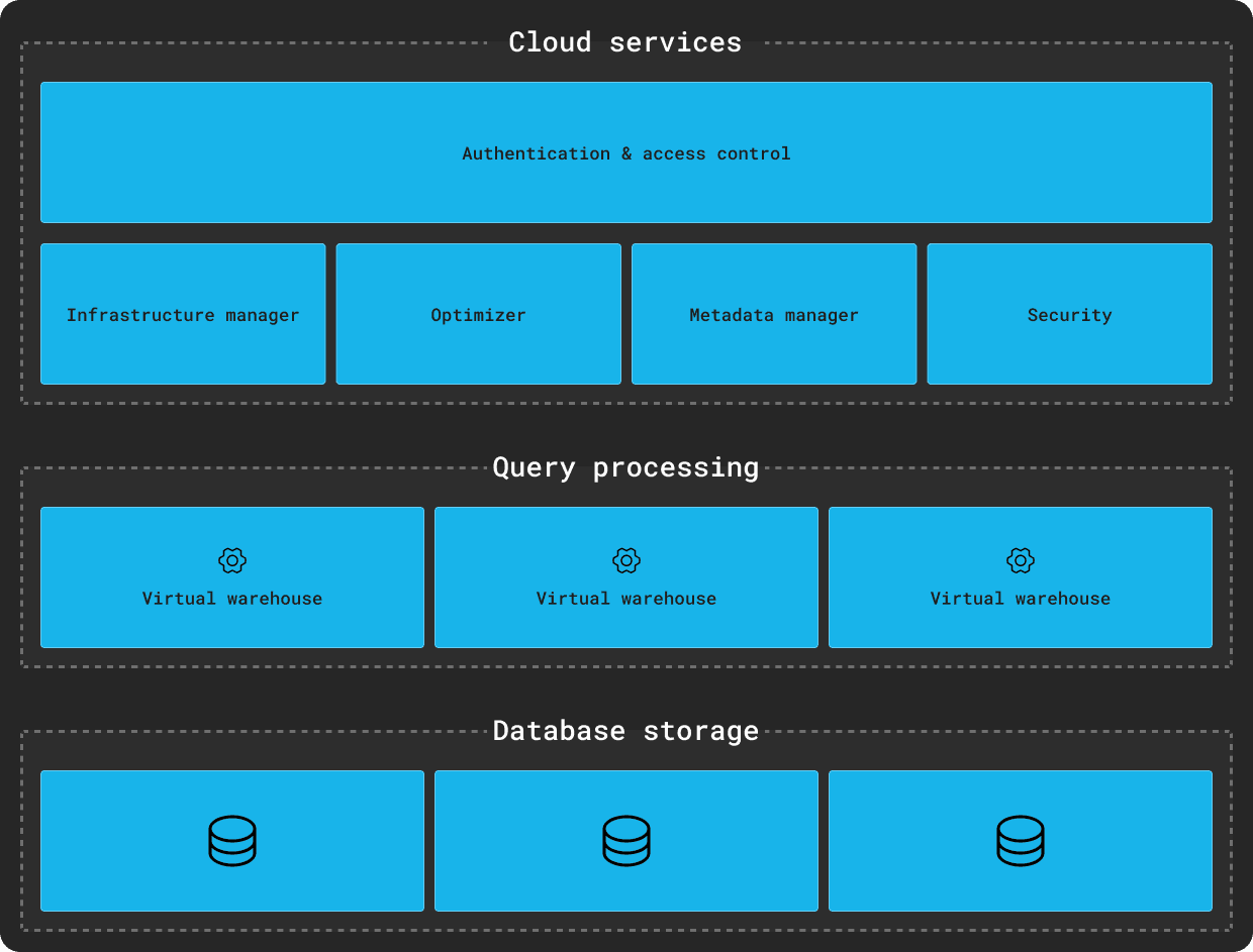 Credit: https://docs.snowflake.com/en/user-guide/intro-key-concepts
Conversely, as an open-source and cloud-hosted product, ClickHouse can be deployed in both shared-disk and shared-nothing architectures. The latter is typical for self-managed deployments. While allowing for CPU and memory to be easily scaled, shared-nothing configurations introduce classic data management challenges and overhead of data replication, especially during membership changes.
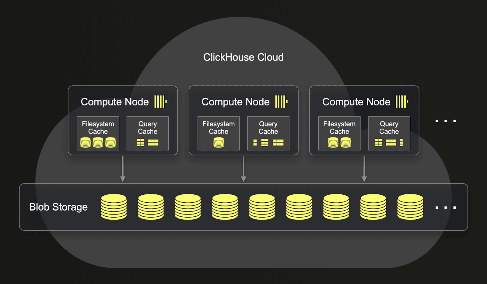
For this reason, ClickHouse Cloud utilizes a shared-storage architecture that is conceptually similar to Snowflake. Data is stored once in an object store (single copy), such as S3 or GCS, providing virtually infinite storage with strong redundancy guarantees. Each node has access to this single copy of the data as well as its own local SSDs for cache purposes. Nodes can, in turn, be scaled to provide additional CPU and memory resources as required. Like Snowflake, S3’s scalability properties address the classic limitation of shared-disk architectures (disk I/O and network bottlenecks) by ensuring the I/O throughput available to current nodes in a cluster is not impacted as additional nodes are added.
Differences
Aside from the underlying storage formats and query engines, these architectures differ in a few subtle ways:
- Compute resources in Snowflake are provided through a concept of warehouses. These consist of a number of nodes, each of a set size. While Snowflake doesn't publish the specific architecture of their warehouses, it is generally understood that each node consists of 8 vCPUs, 16GiB, and 200GB of local storage (for cache). The number of nodes depends on a t-shirt size, e.g. an x-small has one node, a small 2, medium 4, large 8, etc. These warehouses are independent of the data and can be used to query any database residing on object storage. When idle and not subjected to query load, warehouses are paused - resuming when a query is received. While storage costs are always reflected in billing, warehouses are only charged when active.
- ClickHouse Cloud utilizes a similar principle of nodes with local cache storage. Rather than t-shirt sizes, users deploy a service with a total amount of compute and available RAM. This, in turn, transparently auto-scales (within defined limits) based on the query load - either vertically by increasing (or decreasing) the resources for each node or horizontally by raising/lowering the total number of nodes. ClickHouse Cloud nodes currently have a 1:4 CPU-to-memory ratio, unlike Snowflake's 1:2. While a looser coupling is possible, services are currently coupled to the data, unlike Snowflake warehouses. Nodes will also pause if idle and resume if subjected to queries. Users can also manually resize services if needed.
- ClickHouse Cloud's query cache is currently node specific, unlike Snowflake's, which is delivered at a service layer independent of the warehouse. Nonetheless, the above node cache outperforms Snowflake's based on our benchmarks.
- Snowflake and ClickHouse Cloud take different approaches to scaling to increase query concurrency. Snowflake addresses this through a feature known as multi-cluster warehouses. This feature allows users to add clusters to a warehouse. While this offers no improvement to query latency, it does provide additional parallelization and allows higher query concurrency. ClickHouse achieves this by adding more memory and CPU to a service through vertical or horizontal scaling. We do not explore the capabilities of these services to scale to higher concurrency in this blog, focusing instead on latency, but acknowledge that this work should be done for a complete comparison. However, we would expect ClickHouse to perform well in any concurrency test, with Snowflake explicitly limiting the number of concurrent queries allowed for a warehouse to 8 by default. In comparison, ClickHouse Cloud allows up to 1000 queries to be executed per node.
- Snowflake's ability to switch compute size on a dataset, coupled with fast resume times for warehouses, makes it an excellent experience for ad hoc querying. For data warehouse and data lake use cases, this provides an advantage over other systems.
We provide an additional list of similarities and differences concerning features and data types below.
Real-time analytics
Based on our benchmark analysis, ClickHouse outperforms Snowflake for real-time analytics applications in the following areas:
- Query latency: Snowflake queries have a higher query latency even when clustering is applied to tables to optimize performance. In our testing, Snowflake requires over twice the compute to achieve equivalent ClickHouse performance on queries where a filter is applied that is part of the Snowflake clustering key or ClickHouse primary key. While Snowflake's persistent query cache offsets some of these latency challenges, this is ineffective in cases where the filter criteria are more diverse. This query cache effectiveness can be further impacted by changes to the underlying data, with cache entries invalidated when the table changes. While this is not the case in the benchmark for our application, a real deployment would require the new, more recent data to be inserted. Note that ClickHouse's query cache is node specific and not transactionally consistent, making it better suited to real-time analytics. Users also have granular control over its use with the ability to control its use on a per-query basis, its precise size, whether a query is cached (limits on duration or required number of executions), and whether it is only passively used.
- Lower cost: Snowflake warehouses can be configured to suspend after a period of query inactivity. Once suspended, charges are not incurred. Practically, this inactivity check can only be lowered to 60s. Warehouses will automatically resume, within several seconds, once a query is received. With Snowflake only charging for resources when a warehouse is under use, this behavior caters to workloads that often sit idle, like ad-hoc querying. However, many real-time analytics workloads require ongoing real-time data ingestion and frequent querying that doesn't benefit from idling (like customer-facing dashboards). This means warehouses must often be fully active and incurring charges. This negates the cost-benefit of idling as well as any performance advantage that may be associated with Snowflake's ability to resume a responsive state faster than alternatives. This active state requirement, when combined with ClickHouse Cloud's lower per-second cost for an active state, results in ClickHouse Cloud offering a significantly lower total cost for these kinds of workloads.
- Predictable pricing of features: Features such as materialized views and clustering (equivalent to ClickHouse's ORDER BY) are required to reach the highest levels of performance in real-time analytics use cases. These features incur additional charges in Snowflake, requiring not only a higher tier, which increases costs per credit by 1.5x, but also unpredictable background costs. For instance, materialized views incur a background maintenance cost, as does clustering, which is hard to predict prior to use. In contrast, these features incur no additional cost in ClickHouse Cloud, except additional CPU and memory usage at insert time, typically negligible outside of high insert workload use cases. We have observed in our benchmark that these differences, along with lower query latencies and higher compression, result in significantly lower costs with ClickHouse.
ClickHouse users have also voiced appreciation for the wide-ranging support of real-time analytical capabilities provided by ClickHouse, such as:
- An extensive range of specialized analytical functions shorten and simplify query syntax, e.g. aggregate combinators and array functions, improving the performance and readability of complex queries.
- SQL query syntax that is designed to make analytical queries easier, e.g. ClickHouse does not enforce aliases in the SELECT like Snowflake.
- More specific data types, such as support for enums and numerics with explicit precision. The latter allows users to save on uncompressed memory. Snowflake considers lower precision numerics an alias for the equivalent full precision type.
- Superior file and data formats support, compared to a more limited selection in Snowflake, simplifying the import and export of analytical data.
- Federated querying capabilities, enabling ad-hoc queries against a wide range of data lakes and data stores, including S3, MySQL, PostgreSQL, MongoDB, Delta Lake, and more.
- The ability to specify a custom schema or codec for a column to achieve higher compression rates. This feature allowed us to optimize compression rates in our benchmark.
- Secondary indexes & projections. ClickHouse supports secondary indices, including inverted indices for text matching, as well as projections to allow users to target specific queries for optimization. While projections are conceptually similar to Snowflake materialized views, they are not subject to the same limitations with all aggregate functions supported. The use of projections also does not impact pricing (this causes a tier change in Snowflake multiplying charges by 1.5x) other than the associated overhead of increased storage. We demonstrate the effectiveness of these features in our benchmark analysis.
- Support for materialized views. These are distinct from Snowflake materialized views (which are more comparable to ClickHouse projections) in that they are a trigger that executes on the inserted data only. ClickHouse materialized views have a distinct advantage over projections, specifically:
- The result of the materialized view can be stored in another table. This can be a subset or aggregate of the inserted data and be significantly smaller. Unlike in a projection (or materialized view in Snowflake), the original inserted data does not need to be retained, potentially massively saving storage space. If users only need to store the summarized data, materialized views can provide significant storage and performance gains.
- Support for joins and WHERE filters, unlike projections.
- Materialized views can be chained, i.e. multiple views can execute when data is inserted, each producing its own summarized data form.
Clustering vs Ordering
Both ClickHouse and Snowflake are column-oriented databases. This data orientation is superior to row-wise storage and execution for analytical workloads due to the more effective use of CPU caches and SIMD instructions. Furthermore, it ensures sorted columns can be more efficiently compressed since common compression algorithms can exploit repetitive values. While they have different approaches to data storage, both systems require sorting and indices for optimal read performance. This creates some analogous concepts users can leverage when contrasting and migrating data between the systems, even if the implementation differs.
Central to ClickHouse is the use of sparse indices and sorted data. At table creation time, a user specifies an ORDER BY clause containing a tuple of columns. This explicitly controls how the data is sorted. Generally, these columns should be selected based on the frequent queries and listed in order of increasing cardinality. In addition to controlling the order of data on disk, the ORDER BY also, by default, configures the associated sparse primary index. This can be overridden by the PRIMARY KEY clause. Note that the ORDER BY must include the PRIMARY KEY as a prefix, as the latter assumes the data is sorted (see here for an example of where these might differ). This sparse index relies on the data being sorted on disk and is critical to fast query execution in ClickHouse, by allowing data to be scanned efficiently and skipped if it does not match predicates.
Snowflake, while differing in its on-disk storage structures with micro-partitions, provides a similar concept through clustering. This clause allows users to specify a set of columns that control how data is assigned to micro-partitions, aiming to ensure that data with the same values for these columns are co-located. By also effectively controlling data order on disk, clustering offers similar gains in performance and compression in comparison to ClickHouse’s ORDER BY.
Despite their conceptual similarities, there are a few differences in their implementation which affect subsequent usage:
- ClickHouse sorts data at insert time according to the
ORDER BY, constructing the sparse index as data is written to disk. There is no additional cost and negligible overhead at write time, allowing for appropriate optimization even for fast-changing tables. - Snowflake performs clustering asynchronously, consuming credits in the background to keep the data assigned to the right partitions in a process known as Automatic Clustering. The credits which will be consumed during this process cannot be easily predicted. While appropriate for tables that are queried frequently with multi-TiB of data, Snowflake does not recommend clustering for fast-changing tables. The cardinality of the columns used will heavily impact the overhead of clustering and the consumed credits - Snowflake recommends using expressions (e.g.
to_date) to mitigate this impact. Most important for users, when the clustering occurs is not deterministic, so its benefits will not be available immediately when applied to a table. The process is incremental, with clustering improving over time before stabilizing (assuming no further data is added). - Snowflake allows data to be re-clustered at a potentially high cost. This is possible in Snowflake due to a micro-partitioned approach, whereas in ClickHouse, a complete data rewrite is required.
Irrespective of the above differences, these features are critical to analytical workloads, which require selecting, filtering, and sorting on specific columns with GROUP BY operations to support the building of charts with drill-downs. In both cases, it is important to map the columns used in the respective clauses to the workload. A high percentage of queries should benefit from the clustering / ordering keys, with most queries hitting these columns.
When selecting columns for the ORDER BY and CLUSTER BY clauses, ClickHouse and Snowflake provide similar recommendations:
- Use columns that are actively used in selective filters. Columns used in
GROUP BYoperations can also help with respect to memory. - Try to use columns that have sufficient cardinality to ensure effective pruning of the table, e.g. a column holding the outcome of a coin toss will typically prune < 50% of a table.
- When defining multiple columns, users should try to ensure the columns are ordered from the lowest to highest cardinality. This will typically, in both cases, make filtering on later columns more efficient. While details are not available for Snowflake, we expect this to be similar to why this is important for ClickHouse.
Note: While the above recommendations align, Snowflake does recommend avoiding high cardinality columns in clustering keys. This does not impact ClickHouse, however, and columns such as timestamp are valid choices for an ORDER BY clause.
We have considered these recommendations in our subsequent benchmarks.
Migrating Data
Users looking to migrate data between Snowflake and ClickHouse can use object stores, such as S3, as intermediate storage for transfer. This process relies on using the commands COPY INTO and INSERT INTO SELECT of Snowflake and ClickHouse, respectively. We outline this process below.
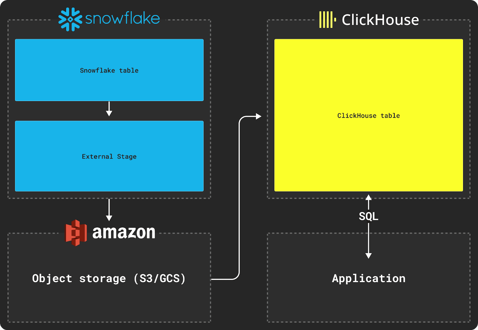
Unloading from Snowflake
Snowflake export requires the use of an External Stage, as shown in the diagram above. This is conceptually similar to a ClickHouse S3 table engine by logically encapsulating a set of externally hosted files and allowing them to be consistently referred to in SQL statements.
We recommend Parquet as the intermittent format when transferring data between systems, principally as it allows type information to be shared, preserves precision, compresses well, and natively supports nested structures common in analytics. Users can also unload to JSON in ndjson format - this is supported in ClickHouse through JSONEachRow, but this is typically significantly more verbose and is larger when decompressed.
In the examples below, we unload 65b rows of the PyPi dataset. This schema and dataset, which originates from a public BigQuery table, is described in greater detail in our benchmarks. This dataset consists of a row for every Python package downloaded, using tools such as PiP. This dataset was selected for its size (>550b rows for all data) as well as having a schema and structure similar to those encountered in real-time analytics use cases.
In the example below, we create a named file format in Snowflake to represent Parquet and the desired file options. This is then used when declaring an external stage with which the COPY INTO command will be used. This provides an abstraction for an S3 bucket through which privileges can be granted.
Note that Snowflake provides several ways to share credentials for write access to an S3 bucket. While we have used option 3, which uses a key and secret directly when declaring the stage to keep the below example simple, the Snowflake Storage Integration approach is recommended in production to avoid the sharing of credentials.
CREATE FILE FORMAT my_parquet_format TYPE = parquet;

CREATE OR REPLACE STAGE my_ext_unload_stage
URL='s3://datasets-documentation/pypi/sample/'
CREDENTIALS=(AWS_KEY_ID='<key>' AWS_SECRET_KEY='<secret>')
FILE_FORMAT = my_parquet_format;

-- apply pypi prefix to all files and specify a max size of 150mb
COPY INTO @my_ext_unload_stage/pypi from pypi max_file_size=157286400 header=true;
The Snowflake schema:
CREATE TABLE PYPI (
   timestamp TIMESTAMP,
   country_code varchar,
   url varchar,
   project varchar,
   file OBJECT,
   installer OBJECT,
   python varchar,
   implementation OBJECT,
   distro VARIANT,
   system OBJECT,
   cpu varchar,
   openssl_version varchar,
   setuptools_version varchar,
   rustc_version varchar,
   tls_protocol varchar,
   tls_cipher varchar
) DATA_RETENTION_TIME_IN_DAYS = 0;
When exported to Parquet, it produces 5.5TiB of data with a maximum file size of 150MiB. A 2X-LARGE warehouse located in the same AWS us-east-1 region takes around 30 mins. The header=true parameter here is required to get column names. The VARIANT and OBJECT columns will also be output as JSON strings by default, forcing us to cast these when inserting them into ClickHouse.
Importing to ClickHouse
Once staged in intermediary object storage, ClickHouse functions such as the s3 table function can be used to insert the data into a table, as shown below.
Assuming the following table target schema:
CREATE TABLE default.pypi
(
	`timestamp` DateTime64(6),
	`date` Date MATERIALIZED timestamp,
	`country_code` LowCardinality(String),
	`url` String,
	`project` String,
	`file` Tuple(filename String, project String, version String, type Enum8('bdist_wheel' = 0, 'sdist' = 1, 'bdist_egg' = 2, 'bdist_wininst' = 3, 'bdist_dumb' = 4, 'bdist_msi' = 5, 'bdist_rpm' = 6, 'bdist_dmg' = 7)),
	`installer` Tuple(name LowCardinality(String), version LowCardinality(String)),
	`python` LowCardinality(String),
	`implementation` Tuple(name LowCardinality(String), version LowCardinality(String)),
	`distro` Tuple(name LowCardinality(String), version LowCardinality(String), id LowCardinality(String), libc Tuple(lib Enum8('' = 0, 'glibc' = 1, 'libc' = 2), version LowCardinality(String))),
	`system` Tuple(name LowCardinality(String), release String),
	`cpu` LowCardinality(String),
	`openssl_version` LowCardinality(String),
	`setuptools_version` LowCardinality(String),
	`rustc_version` LowCardinality(String),
	`tls_protocol` Enum8('TLSv1.2' = 0, 'TLSv1.3' = 1),
	`tls_cipher` Enum8('ECDHE-RSA-AES128-GCM-SHA256' = 0, 'ECDHE-RSA-CHACHA20-POLY1305' = 1, 'ECDHE-RSA-AES128-SHA256' = 2, 'TLS_AES_256_GCM_SHA384' = 3, 'AES128-GCM-SHA256' = 4, 'TLS_AES_128_GCM_SHA256' = 5, 'ECDHE-RSA-AES256-GCM-SHA384' = 6, 'AES128-SHA' = 7, 'ECDHE-RSA-AES128-SHA' = 8)
)
ENGINE = MergeTree
ORDER BY (date, timestamp)
With nested structures such as file converted to JSON strings by Snowflake, importing this data thus requires us to transform these structures to appropriate Tuples at insert time in ClickHouse, using the JSONExtract function as shown below.
INSERT INTO pypi
SELECT
	TIMESTAMP,
	COUNTRY_CODE,
	URL,
	PROJECT,
	JSONExtract(ifNull(FILE, '{}'), 'Tuple(filename String, project String, version String, type Enum8(\'bdist_wheel\' = 0, \'sdist\' = 1, \'bdist_egg\' = 2, \'bdist_wininst\' = 3, \'bdist_dumb\' = 4, \'bdist_msi\' = 5, \'bdist_rpm\' = 6, \'bdist_dmg\' = 7))') AS file,
	JSONExtract(ifNull(INSTALLER, '{}'), 'Tuple(name LowCardinality(String), version LowCardinality(String))') AS installer,
	PYTHON,
	JSONExtract(ifNull(IMPLEMENTATION, '{}'), 'Tuple(name LowCardinality(String), version LowCardinality(String))') AS implementation,
	JSONExtract(ifNull(DISTRO, '{}'), 'Tuple(name LowCardinality(String), version LowCardinality(String), id LowCardinality(String), libc Tuple(lib Enum8(\'\' = 0, \'glibc\' = 1, \'libc\' = 2), version LowCardinality(String)))') AS distro,
	JSONExtract(ifNull(SYSTEM, '{}'), 'Tuple(name LowCardinality(String), release String)') AS system,
	CPU,
	OPENSSL_VERSION,
	SETUPTOOLS_VERSION,
	RUSTC_VERSION,
	TLS_PROTOCOL,
	TLS_CIPHER
FROM s3('https://datasets-documentation.s3.eu-west-3.amazonaws.com/pypi/2023/pypi*.parquet')
SETTINGS input_format_null_as_default = 1, input_format_parquet_case_insensitive_column_matching = 1
We rely on the settings input_format_null_as_default=1 and input_format_parquet_case_insensitive_column_matching=1 here to ensure columns are inserted as default values if null, and column matching between the source data and target table is case insensitive.
If using Azure or Google Cloud, similar processes can be created. Note dedicated functions exist in ClickHouse[1][2] for importing data from these object stores.
Conclusion
In this post, we have contrasted Snowflake and ClickHouse for the real-time analytics use case, looking at similarities and differences between the systems. We have identified ClickHouse features beneficial to this use case and explored how users might migrate workloads from Snowflake. In the next post in this series, we will introduce a sample real-time analytics application, identify differences in compression and insert performance, and benchmark representative queries. This will conclude with a cost analysis where we present possible savings with ClickHouse Cloud.
Appendix
Users looking to migrate real-time analytics workloads from Snowflake to ClickHouse may need to understand several key concepts. Below, we provide additional information on data types and equivalences in core clustering and ordering. This information supplements the earlier section on the high-level approach to transferring data.
Data Types
Numerics
Users moving data between ClickHouse and Snowflake will immediately notice that ClickHouse offers more granular precision concerning declaring numerics. For example, Snowflake offers the type Number for numerics. This requires the user to specify a precision (total number of digits) and scale (digits to the right of the decimal place) up to a total of 38. Integer declarations are synonymous with Number, and simply define a fixed precision and scale where the range is the same. This convenience is possible as modifying the precision (scale is 0 for ints) does not impact the size of data on disk in Snowflake - the minimal required bytes are used for a numeric range at write time at a micro partition level. The scale does, however, impact storage space and is offset with compression. A Float64 type offers a wider range of values with a loss of precision.
Contrast this with ClickHouse, which offers multiple signed and unsigned precisions for floats and ints. With these, ClickHouse users can be explicit about the precision required for integers to optimize storage and memory overhead. A Decimal type, equivalent to Snowflake’s Number type, also offers twice the precision and scale at 76 digits. In addition to a similar Float64 value, ClickHouse also provides a Float32 for when precision is less critical and compression paramount.
Strings
ClickHouse and Snowflake take contrasting approaches to the storage of string data. The VARCHAR in Snowflake holds Unicode characters in UTF-8, allowing the user to specify a maximum length. This length has no impact on storage or performance, with the minimum number of bytes always used to store a string, and rather provides only constraints useful for downstream tooling. Other types, such as Text and NChar, are simply aliases for this type. ClickHouse conversely stores all string data as raw bytes with a String type (no length specification required), deferring encoding to the user, with query time functions available for different encodings (see here for motivation). The ClickHouse String is thus more comparable to the Snowflake Binary type in its implementation. Both Snowflake and ClickHouse support “collation”, allowing users to override how strings are sorted and compared.
Semi-structured
Snowflake and ClickHouse are comparable with rich type support for semi-structured data, providing such support through the VARIANT (a supertype in effect) and JSON types, respectively. These types allow “schema-later” with the underlying data types identified at insert time by the database. Snowflake also supports the ARRAY and OBJECT types, but these are just restrictions of type VARIANT.
ClickHouse also supports named Tuples and arrays of Tuples via the Nested type, allowing users to explicitly map nested structures. This allows codecs and type optimizations to be applied throughout the hierarchy, unlike Snowflake, which requires the user to use the OBJECT, VARIANT, and ARRAY types for the outer object and does not allow explicit internal typing. This internal typing also simplifies queries on nested numerics in ClickHouse, which do not need to be cast and can be used in index definitions.
In ClickHouse, codecs and optimized types can also be applied to sub-structures. This provides an added benefit that compression with nested structures remains excellent, and comparable, to flattened data. In contrast, as a result of the inability to apply specific types to sub structures, Snowflake recommends flattening data in order to achieve optimal compression. Snowflake also imposes size restrictions for these data types.
Below we map the equivalent types for users migrating workloads from Snowflake to ClickHouse:
| Snowflake | ClickHouse | Note |
|---|---|---|
| NUMBER | Decimal | ClickHouse supports twice the precision and scale than Snowflake - 76 digits vs. 38. |
| FLOAT, FLOAT4, FLOAT8 | Float32, Float64 | All floats in Snowflake are 64 bit. |
| VARCHAR | String | |
| BINARY | String | |
| BOOLEAN | Bool | |
| DATE | Date, Date32 | DATE in Snowflake offers a wider date range than ClickHouse e.g. min for Date32 is 1900-01-01 and Date 1970-01-01. Date in ClickHouse provides more cost efficient (two byte) storage. |
| TIME(N) | No direct equivalent but can be represented by DateTime and DateTime64(N). | DateTime64 uses the same concepts of precision. |
| TIMESTAMP - TIMESTAMP_LTZ, TIMESTAMP_NTZ, TIMESTAMP_TZ | DateTime and DateTime64 | DateTime and DateTime64 can optionally have a TZ parameter defined for the column. If not present, the server's timezone is used. Additionally a --use_client_time_zone parameter is available for the client. |
| VARIANT | JSON, Tuple, Nested | JSON type is experimental in ClickHouse. This type infers the column types at insert time. Tuple, Nested and Array can also be used to build explicitly type structures as an alternative. |
| OBJECT | Tuple, Map, JSON | Both OBJECT and Map are analogous to JSON type in ClickHousewhere the keys are a String. ClickHouse requires the value to be consistent and strongly typed whereas Snowflake uses VARIANT. This means the values of different keys can be a different type. If this is required in ClickHouse, explicitly define the hierarchy using Tuple or rely on JSON type. |
| ARRAY | Array, Nested | ARRAY in Snowflake uses VARIANT for the elements - a super type. Conversely these are strongly typed in ClickHouse. |
| GEOGRAPHY | Point, Ring, Polygon, MultiPolygon | Snowflake imposes a coordinate system (WGS 84) while ClickHouse applies at query time. |
| GEOMETRY | Point, Ring, Polygon, MultiPolygon |
- IP-specific types ipv4 and ipv6, potentially allowing more efficient storage than Snowflake.
- FixedString - allows a fixed length of bytes to be used, which is useful for hashes.
- LowCardinality - allows any type to be dictionary encoded. Useful for when the cardinality is expected to be < 100k.
- Enum - allows efficient encoding of named values in either 8 or 16-bit ranges.
- UUID for efficient storage of uuids.
- Vectors can be represented as an Array of Float32 with supported distance functions.
Finally, ClickHouse offers the unique ability to store the intermediate state of aggregate functions. This state is implementation-specific, but allows the result of an aggregation to be stored and later queried (with corresponding merge functions). Typically, this feature is used via a materialized view and, as demonstrated below, offers the ability to rapidly accelerate specific queries with minimal storage cost by storing the incremental result of queries over inserted data (more details here).
Contact us today to learn more about real-time analytics with ClickHouse Cloud. Or, get started with ClickHouse Cloud and receive $300 in credits.