Summary
This ClickHouse vs. Snowflake blog series consists of two parts which can be read independently. The parts are as follows.
- Benchmarks and Cost Analysis - In this post, we benchmark a set of real-time analytics queries that would power a proposed application. These queries are evaluated in both systems, using a wide range of optimizations, and the cost is compared directly.
- Comparing and Migrating - This post focuses on outlining the architectural similarities and differences between the ClickHouse and Snowflake, and reviews the features that are particularly well-suited for the real-time analytics use case in ClickHouse Cloud. For users interested in migrating workloads from Snowflake to ClickHouse, we explore differences in datasets and a means of migrating data.
Table of Contents
Introduction
In this post, we provide an example of a real-time analytics application that has the ability to analyze downloads for Python packages over time. This application is powered by the PyPI dataset, which consists of almost 600 billion rows.
We identify representative queries to power a real-time application, benchmark the performance of both ClickHouse and Snowflake using this workload, and perform an analysis of the costs – the cost of running the benchmark itself, as well as the projected ongoing cost of running the application in production.
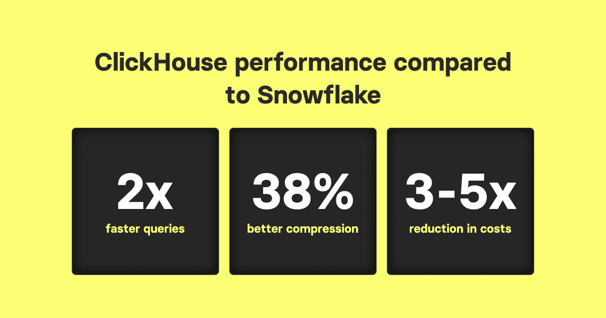
Based on this analysis, we believe ClickHouse can provide significant performance and cost improvements compared to Snowflake for real-time analytics use cases. Our results show that:
- ClickHouse Cloud is 3-5x more cost-effective than Snowflake in production.
- ClickHouse Cloud querying speeds are over 2x faster compared to Snowflake.
- ClickHouse Cloud results in 38% better data compression than Snowflake.
The information and methodology needed to replicate this benchmark analysis is also publicly available at https://github.com/ClickHouse/clickhouse_vs_snowflake.
Benchmarks
In the following section, we compare the insert and query performance for ClickHouse and Snowflake, as well as the compression achieved, for the queries of a proposed application. For all tests, we use GCE-hosted instances in us-central-1 since the test dataset below is most easily exported to GCS.
We use production instances of a ClickHouse Cloud service for our examples with a total of 177, 240, and 256 vCPUs. For Snowflake, we have predominantly used either a 2X-LARGE or 4X-LARGE cluster, which we believe to possess 256 and 512 vCPUs (it is generally understood that each node consists of 8 vCPUs, 16GiB, and 200GB of local storage), respectively - the former representing the closest configuration to our ClickHouse clusters. While some of the Snowflake configurations provide an obvious compute advantage over the above ClickHouse clusters, ClickHouse Cloud has a greater cpu:memory ratio (1:4 for ClickHouse vs. 1:2 for Snowflake) offsetting some of this advantage; however, the offset is not significant for this benchmark because the queries are not memory-intensive.
For users looking to reproduce our results, we note that these configurations can be expensive to test in Snowflake - for example, loading the dataset into Snowflake cost us around $1100, with clustering optimizations applied, as compared to about $40 in ClickHouse Cloud. Users can choose to load subsets to reduce this cost and/or run a limited number of benchmarks. On the ClickHouse side, if desired, these examples should be reproducible on an equivalently sized self-managed ClickHouse cluster, if usage of ClickHouse Cloud is not possible.
Application & dataset
PyPI dataset
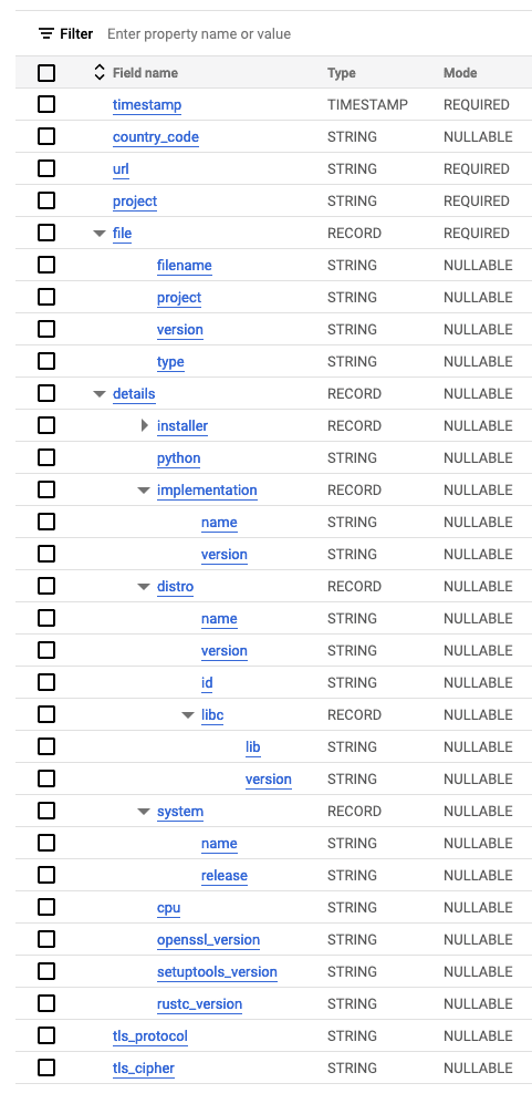
The PyPI dataset is currently available as a public table in BigQuery. Each row in this dataset represents one download of a Python package by a user (using pip or similar technique). We have exported this data as Parquet files, making it available in the public GCS bucket gcs://clickhouse_public_datasets/pypi/file_downloads. The steps for this are available here. The original schema for this dataset is shown below. Due to the nested structures, Parquet was chosen as the optimal export format that Snowflake and ClickHouse support.
By default, the export file size is determined by the partitioning in BigQuery. The full export of 560 billion rows in the above GCS folder consists of 19TiB of Parquet split over 1.5 million files. While easily importable into ClickHouse, these small files are problematic when importing into Snowflake (see below).
In order to provide a more cost-viable subset for our tests, we exported only the last three months as of 23/06/2023. To conform to Snowflake's best practices when loading Parquet files, we targeted file sizes between 100MiB and 150MiB. To achieve this, BigQuery requires the table to be copied and re-partitioned before exporting. Using the steps here, we were able to export 8.74TiB of data as 70,608 files with an average size of 129MiB.
Proposed application
For the purposes of this benchmark analysis, we compare queries that could be used to build a simple analytics service where users can enter a package name and retrieve a selection of interesting trends, ideally rendered as charts, for the package. This includes, but is not limited to:
- Downloads over time, rendered as a line chart.
- Downloads over time per Python version, rendered as a multi-series line chart.
- Downloads over time per system, e.g. Linux, rendered as a multi-series bar chart.
- Top distribution/file types for the project, e.g. sdist or bdist, rendered as a pie or bar chart.
In addition, the application might allow the user to identify:
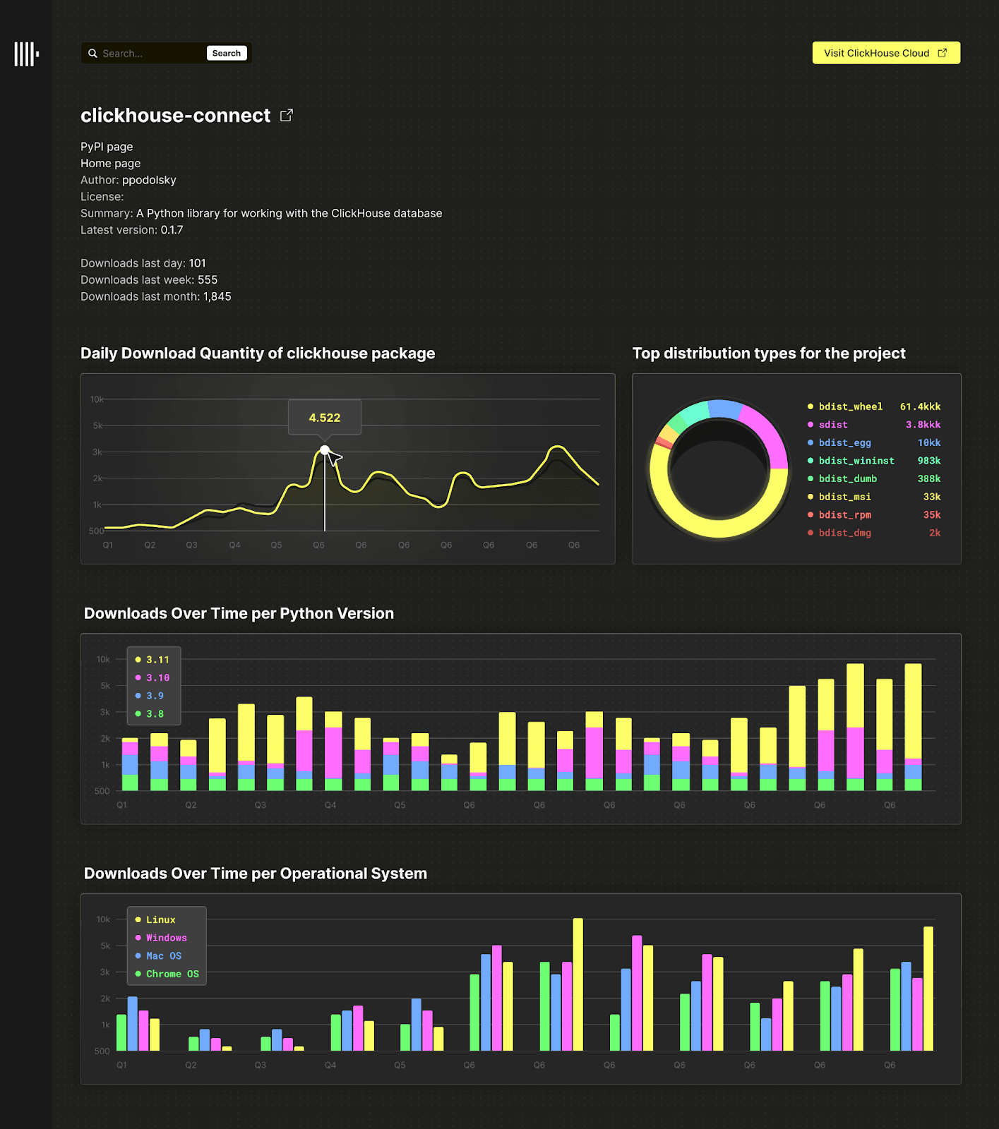
- Total downloads for related sub-projects (if they exist) for a technology, e.g.
clickhouse-connectfor ClickHouse. - Top projects for a specific distro, e.g. Ubuntu.
This might look something like the following:
The above represents a straightforward real-time application with many enhancement possibilities. While many real-time analytics applications are more complex than this, the above allows us to model the query workload fairly easily. Assuming we also allow the user to drill down on a date period, updating the charts, we can evaluate the query performance of both Snowflake and ClickHouse for this application.
In our benchmark, we model this workload in its simplest form. We devise a SQL query for each chart representing the initial rendering when a user types a project name into the search box. A subsequent query then filters the chart on a randomly generated date range to simulate the interactive use of the application. Queries for both systems use the same dates and projects, executed in the same order, for fairness. We execute these queries with a single thread, one after another (focusing on absolute latency). It does not test a workload with concurrent requests; neither does it test for system capacity. While we would expect ClickHouse to perform well under highly concurrent workloads, this test is significantly more complex to execute fairly and interpret results from.
Assumptions & limitations
In effort to make this benchmark easy to reproduce with a high number of configurations, and the results simple to interpret, we made some assumptions to constrain the scope of the exercise. A full list of assumptions and limitations can be found here, but most notably:
- We did not evaluate Snowflake's multi-cluster warehouse feature. While not applicable to our test workload, this would be invaluable in scaling throughput for a production application. The approach has merits and contrasts with ClickHouse Cloud, where services are scaled by adding nodes.
- Snowflake's persistent cache adds significant value. In addition to being robust to warehouse restarts, the cache is fully distributed and independent of warehouses. This ensures a high rate of cache hits. While ClickHouse Cloud has a query cache faster than Snowflake’s, it is currently per node (although a distributed cache is planned).
- We have not evaluated the query acceleration service from Snowflake. This service offloads query processing work to shared compute resources for specific queries at significant additional cost. However, Snowflake states that query acceleration service depends on server availability and performance improvements might fluctuate over time, making it not a great fit for reproducible benchmarks.
Schemas
ClickHouse
Our ClickHouse schema is shown below:
CREATE TABLE default.pypi
(
   `timestamp` DateTime64(6),
   `date` Date MATERIALIZED timestamp,
   `country_code` LowCardinality(String),
   `url` String,
   `project` String,
   `file` Tuple(filename String, project String, version String, type Enum8('bdist_wheel' = 0, 'sdist' = 1, 'bdist_egg' = 2, 'bdist_wininst' = 3, 'bdist_dumb' = 4, 'bdist_msi' = 5, 'bdist_rpm' = 6, 'bdist_dmg' = 7)),
   `installer` Tuple(name LowCardinality(String), version LowCardinality(String)),
   `python` LowCardinality(String),
   `implementation` Tuple(name LowCardinality(String), version LowCardinality(String)),
   `distro` Tuple(name LowCardinality(String), version LowCardinality(String), id LowCardinality(String), libc Tuple(lib Enum8('' = 0, 'glibc' = 1, 'libc' = 2), version LowCardinality(String))),
   `system` Tuple(name LowCardinality(String), release String),
   `cpu` LowCardinality(String),
   `openssl_version` LowCardinality(String),
   `setuptools_version` LowCardinality(String),
   `rustc_version` LowCardinality(String),
   `tls_protocol` Enum8('TLSv1.2' = 0, 'TLSv1.3' = 1),
   `tls_cipher` Enum8('ECDHE-RSA-AES128-GCM-SHA256' = 0, 'ECDHE-RSA-CHACHA20-POLY1305' = 1, 'ECDHE-RSA-AES128-SHA256' = 2, 'TLS_AES_256_GCM_SHA384' = 3, 'AES128-GCM-SHA256' = 4, 'TLS_AES_128_GCM_SHA256' = 5, 'ECDHE-RSA-AES256-GCM-SHA384' = 6, 'AES128-SHA' = 7, 'ECDHE-RSA-AES128-SHA' = 8)
)
ENGINE = MergeTree
ORDER BY (project, date, timestamp)
We apply a number of type optimizations here as well as adding the materialized column date to the schema. This is not part of the raw data and has been added purely for use in the primary key and filter queries. We have represented the nested structures file, installer, implementation, and distro as named tuples. These are hierarchical data structures (rather than fully semi-structured) and thus have predictable sub-columns. This allows us to apply the same type of optimizations as those applied to root columns.
Full details on the optimizations applied can be found here.
Snowflake
Our Snowflake schema:
CREATE TRANSIENT TABLE PYPI (
   timestamp TIMESTAMP,
   country_code varchar,
   url varchar,
   project varchar,
   file OBJECT,
   installer OBJECT,
   python varchar,
   implementation OBJECT,
   distro VARIANT,
   system OBJECT,
   cpu varchar,
   openssl_version varchar,
   setuptools_version varchar,
   rustc_version varchar,
   tls_protocol varchar,
   tls_cipher varchar
) DATA_RETENTION_TIME_IN_DAYS = 0;
Snowflake does not require VARCHAR columns to have a limit specified, with no performance or storage penalty, simplifying the declaration significantly. We optimize the schema by declaring the table as TRANSIENT and disabling time travel (DATA_RETENTION_TIME_IN_DAYS = 0). The former turns off Snowflake’s fail-safe feature, which retains a copy of the data for seven days for emergency recovery, which is not required in our case and reduces costs. ClickHouse Cloud supports backups, providing a similar function to failsafe - these are incorporated into the storage cost. While powerful, the time travel feature, which allows historical data to be queried, is not required for our real-time analytics.
An astute reader will have noticed the above schemas are not the same as the original BigQuery schema, which has an additional level of nesting with some columns underneath a
detailscolumn. We have removed this extra level at export time to simplify the schema for both ClickHouse and Snowflake. This makes subsequent queries simpler.
Initially we have not specified a clustering key, but we do it in further experiments, once data is loaded.
Results
These tests were performed on ClickHouse 23.6, unless stated, and in the first 2 weeks of June for Snowflake.
Summary
Based on our benchmarking results, we can draw the following conclusions when comparing Snowflake and ClickHouse's performance for this scenario:
- ClickHouse offers up to 38% better compression than the best offered by Snowflake with clustering enabled.
- Clustering in Snowflake improves compression by up to 45% in our tests. This feature appears essential for query performance to be remotely competitive with ClickHouse, especially when filtering on ordering keys. However, it comes at significant costs due to the background processes responsible for ordering the data.
- ClickHouse is up to 2x faster at loading data than Snowflake, even with a comparable number of vCPUs and when ignoring the time required for Snowflake to cluster data. This also assumes file sizes are optimal for Snowflake - it appears to perform significantly worse on smaller files.
- A workload where queries can exploit a clustering/ordering key is the most common in real-time analytics use cases. In this scenario, ClickHouse is 2-3x faster for hot queries than a Snowflake warehouse which has more vCPUs (177 vs. 256) and is configured with an equivalent optimized clustering key. This performance difference is maintained across all tests, even when aggregating by columns on which the ClickHouse and Snowflake tables are not ordered/clustered by.
- The difference in cold queries is less dramatic, but ClickHouse still outperforms Snowflake by 1.5 to 2x. Furthermore, clustering comes at a significant additional cost. For further details, also see Cost analysis.
- Materialized views in Snowflake are comparable to ClickHouse projections, albeit with more restrictions, and offer strong performance gains for queries. For our limited workload, these offered greater improvement than projections, even still, mean performance is 1.5x slower than ClickHouse.
- Snowflake is around 30% faster than ClickHouse on GROUP BY queries which cannot efficiently exploit ordering/clustering keys and are forced to scan more data. This can partially be attributed to the higher number of vCPUs but also its ability to distribute work across nodes efficiently. The equivalent feature in ClickHouse, parallel replicas, is currently experimental and subject to further improvements.
- For queries that require full table scans, such as LIKE, Snowflake offers more consistent query performance with lower 95/99th percentiles than ClickHouse, but higher mean performance.
- Secondary indices in ClickHouse are comparable in performance for LIKE queries to Snowflakes Search Optimization Service, with better hot performance, but slightly slower cold performance. Whereas this feature in ClickHouse adds minimal cost, with only slightly raised storage, it adds significant expense in Snowflake - see Cost analysis.
Full results are detailed below.
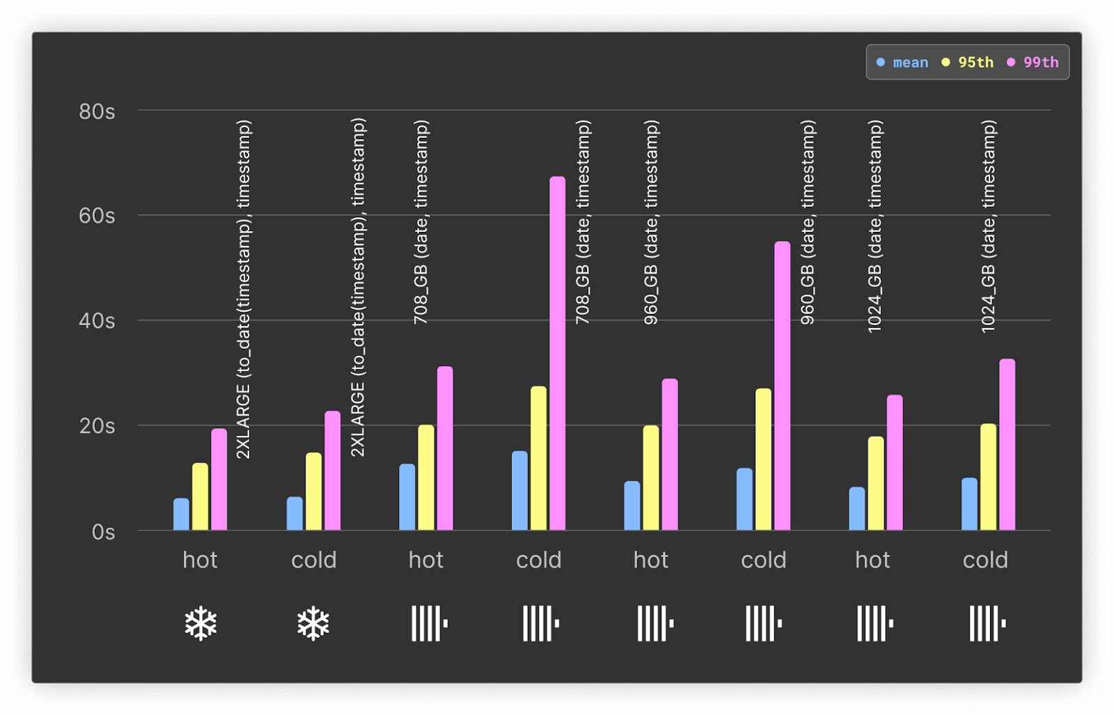
Data loading
To evaluate the load performance of ClickHouse and Snowflake, we tested several service and warehouse sizes with comparable CPU and memory resources.
Full details of data loading and the commands used can be found here. We have optimized insert performance into both ClickHouse and Snowflake. With the former, we use a number of settings focused on distributing inserts and ensuring data is written in large batches. For Snowflake, we have followed documented best practices and ensured Parquet files are around 150MiB.
To improve ClickHouse insert performance, we tuned the number of threads as noted here. This causes a large number of parts to be formed, which must be merged in the background. High part counts negatively impact SELECT performance, so we report the total time taken for merges to reduce the part count to under 3000 (default recommended total) - queries for this here. This is the value compared to Snowflake’s total load time.
| Database | Specification | Number of nodes | Memory per node (GiB) | vCPUs per node | Total vCPUs | Total memory (GiB) | Insert threads | Total time (s) |
|---|---|---|---|---|---|---|---|---|
| Snowflake | 2X-LARGE | 32 | 16 | 8 | 256 | 512 | NA | 11410 |
| Snowflake | 4X-LARGE | 128 | 16 | 8 | 1024 | 2048 | NA | 2901 |
| ClickHouse | 708GB | 3 | 236 | 59 | 177 | 708 | 4 | 15370 |
| ClickHouse | 708GB | 3 | 236 | 59 | 177 | 708 | 8 | 10400 |
| ClickHouse | 708GB | 3 | 236 | 59 | 177 | 708 | 16 | 11400 |
| ClickHouse | 1024GB | 16 | 64 | 16 | 256 | 1024 | 1* | 9459 |
| ClickHouse | 1024GB | 16 | 64 | 16 | 256 | 1024 | 2 | 5730 |
| ClickHouse | 960GB | 8 | 120 | 30 | 240 | 960 | 4 | 6110 |
| ClickHouse | 960GB | 8 | 120 | 30 | 240 | 960 | 8 | 5391 |
| ClickHouse | 960GB | 8 | 120 | 30 | 240 | 960 | 16 | 6133 |
If we compare the best results for a 2X-LARGE (256 vCPUs) vs. 960GB (240 vCPUs), which have similar resources, ClickHouse delivers over 2x the insert performance of Snowflake for the same number of vCPUs.
Other observations from this test:
-
On clusters with fewer nodes but more vCPUs per node (e.g. 708GB configuration), ClickHouse completes the initial insert operation faster. However, time is then spent merging parts below an acceptable threshold. While multiple merges can occur on a node at any time, the total number per node is limited. Spreading our resources across more nodes (960GB has 8 x 30 core nodes), allows more concurrent merges to occur, resulting in a faster completion time (these higher levels of configurations can be requested in ClickHouse Cloud by contacting support).
-
To achieve maximum load performance, Snowflake needs as many files as vCPUs. We hypothesize this is because reading within Parquet files is not parallelized, unlike ClickHouse. While this is not an issue on our dataset, this makes scaling inserts challenging in other scenarios.
-
Snowflake recommends ensuring Parquet files are around 150MiB. The full PyPi dataset, consisting of over 1.5M files and 19TiB, has a much smaller average file size of 13MiB. Since we did not expect ClickHouse to be appreciably impacted by file size, we followed Snowflake’s recommendation of 150MiB.
To test the differences in behavior on small Parquet files, we imported a 69B row sample of the PyPi dataset into both ClickHouse and Snowflake. This sample, which consists of exactly 3 months of data, can be found under the bucket
gs://clickhouse_public_datasets/pypi/file_downloads/2023_may_aug/and consists of 1.06TiB of Parquet split over 109,448 files for an average size of 10MiB. While Snowflake total load time does not appear to be appreciably impacted by these smaller file sizes, ClickHouse actually benefits and outperforms Snowflake by ~35%. While this test was conducted on a later version of ClickHouse 23.8, further testing does suggest ClickHouse is faster on 10MiB files vs. 150MiB. We did not test other file sizes. Full results can be found here.
- Snowflake exhibits linear improvements in load time to the number of vCPUs. This means the total cost to the user remains constant, i.e. a 4X-LARGE warehouse is twice the cost of a 2X-LARGE, but the load time is half. The user can, in turn, make the warehouse idle on completion, incurring the same total charge. ClickHouse Cloud’s new feature, SharedMergeTree, also ensures insert performance scales linearly with resources. While the above benchmark test results use the ClickHouse standard MergeTree, due to when these benchmarks were conducted, examples of results demonstrating linear scalability for SharedMergeTree with this dataset can be found here.
- The above does not include any clustering time for Snowflake. Clustering, as shown below, is required for query performance to be competitive with ClickHouse. However, if clustering times are included in the comparison, Snowflake insert times become significantly higher than ClickHouse - this is challenging to measure precisely, as clustering is asynchronous, and its scheduling is non-deterministic.
Further observations from this test can be found here.
Storage efficiency & compression
Our earlier ClickHouse schema is mostly optimized for maximum compression. As shown below, it can be further improved by applying a delta codec to the date and timestamp columns, although this was shown to have side effects concerning performance on cold queries.
By default, a Snowflake schema does not include clustering. Clustering is configured by setting the clustering key, the choice of which heavily impacts data compression. In order to thoroughly evaluate Snowflake compression rates, we’ve thus tested various clustering keys and recorded the resulting total compressed data size for each, illustrated below.
Full details on our compression results and how this was measured can be found here.
| Database | ORDER BY/CLUSTER BY | Total size (TiB) | Compression ratio on Parquet |
|---|---|---|---|
| Snowflake | - | 1.99 | 4.39 |
| Snowflake | (to_date(timestamp), project) | 1.33 | 6.57 |
| Snowflake | (project) | 1.52 | 5.75 |
| Snowflake | (project, to_date(timestamp)) | 1.77 | 4.94 |
| Snowflake | (project, timestamp)* | 1.05 | 8.32 |
| ClickHouse | (project, date, timestamp) | 0.902 | 9.67 |
| ClickHouse | (project, date, timestamp) + delta codec | 0.87 | 10.05 |
| Most optional query performance |
| Most optimal compression |
Note that we were unable to identify an uncompressed size for Snowflake and are unable to provide a compression ratio similar to ClickHouse. We have thus computed a compression ratio to Parquet.
Clustering in Snowflake is essential for good compression and query performance in our use case. The best clustering key chosen for our Snowflake schema resulted in reducing the data size by 40%. Despite including the extra column date, the best compression in ClickHouse is nonetheless better than the most optimal Snowflake configuration by almost 20% (0.87TiB vs. 1.05TiB).
That said, the best-performing clustering key for Snowflake, with respect to compression, did not result in the best Snowflake query performance. Snowflake users are therefore presented with a tradeoff – optimize for compression (and thus storage costs) or have faster queries.
For our benchmark analysis, the objective is to support a real-time analytics workload, for which fast querying is essential. Therefore, the clustering key used for the remainder of our benchmarks is the clustering key that benefits querying speed over compression, and also adheres to Snowflake’s published best practices which recommends the lower cardinality column first. This is the (to_date(timestamp), project) clustering key.
Based on the configurations and schemas optimized for query speed, our results show that ClickHouse Cloud outperforms Snowflake in compression by 38% (0.902TiB vs. 1.33TiB).
Clustering time & costs in Snowflake
As described by the Snowflake documentation, clustering incurs tradeoffs. While improving query performance, users will be charged credits by the use of this asynchronous service. We have attempted to capture the total credits (and cost) required for each of the above clustering keys below and the time taken for clustering to stabilize. Time consumed here is an estimate as Snowflake provides only hour-level granularity in its AUTOMATIC_CLUSTERING_HISTORY view. See here for the query used to compute clustering costs.
| CLUSTER BY | Time taken (mins) | Rows clustered | Bytes clustered | Credits used | Total cost (assuming standard) |
|---|---|---|---|---|---|
| (to_date(timestamp), project) | 540 | 53818118911 | 1893068905149 | 450 | $990 |
| (project) | 360 | 41243645440 | 1652448880719 | 283 | $566 |
| (project, to_date(timestamp)) | 180 | 56579552438 | 1315724687124 | 243 | $486 |
| (project, timestamp) | 120 | 50957022860 | 1169499869415 | 149 | $298 |
The timings in the table above can be considered in addition to the insert performance tests. Effective clustering, where a large number of the bytes are clustered, appears to incur a significant cost with respect to credits and time in Snowflake.
The equivalent feature in ClickHouse (using an ORDER BY) incurs no additional charges and it is required by default for all tables. Additional ordering can be added to ClickHouse tables through projections. In this case users pay for additional storage only. Projections and ordering only incur incremental compute and memory overhead to sort data at insert time and perform background merges. CPU and memory used by background processes have a lower priority than queries and usually utilize idle resources on an existing service. Completion of these background operations is not required for queries to run and observe updated data, but improve performance of future queries.
Querying
We simulate a load for each of our proposed visualizations to evaluate query performance. We summarize the results below, providing links to the complete analysis for those wanting to reproduce benchmarks. We assume:
- Clustering has been completed on Snowflake, and the part count is below 3000 in ClickHouse.
- All queries are executed 3 times to obtain cold and hot execution times. We consider the hot result to be the fastest time and the cold the slowest.
- Prior to executing on ClickHouse, we clear any file system caches, i.e. `SYSTEM DROP FILESYSTEM CACHE ON CLUSTER 'default". This does not appear to be possible on Snowflake, so we paused and resumed the warehouse.
- Query caches are disabled for Snowflake and ClickHouse unless stated. The query cache in ClickHouse Cloud is disabled by default. Snowflake's cache is on by default and must be disabled, i.e.
ALTER USER <user> SET USE_CACHED_RESULT = false;. - All queries use an absolute date for the upper bound of the data when computing the last 90 days. This allows the tests to be run at any time and query caches to be exploited (when enabled).
Query 1: Downloads per day
The results of this query are designed to show downloads over time per day, for the last 90 days, for a selected project. For the top 100 projects, a query is issued computing this aggregation. A narrower time filter is then applied to a random time frame (same random values for both databases), grouping by an interval that produces around 100 buckets (so any chart points render sensibly), thus simulating a user drilling down. This results in a total of 200 queries.
SELECT
    toStartOfDay(date),
    count() AS count
FROM pypi
WHERE (project = 'typing-extensions') AND (date >= (CAST('2023-06-23', 'Date') - toIntervalDay(90)))
GROUP BY date
ORDER BY date ASC
The full results, queries and observations can be found here.
Hot only
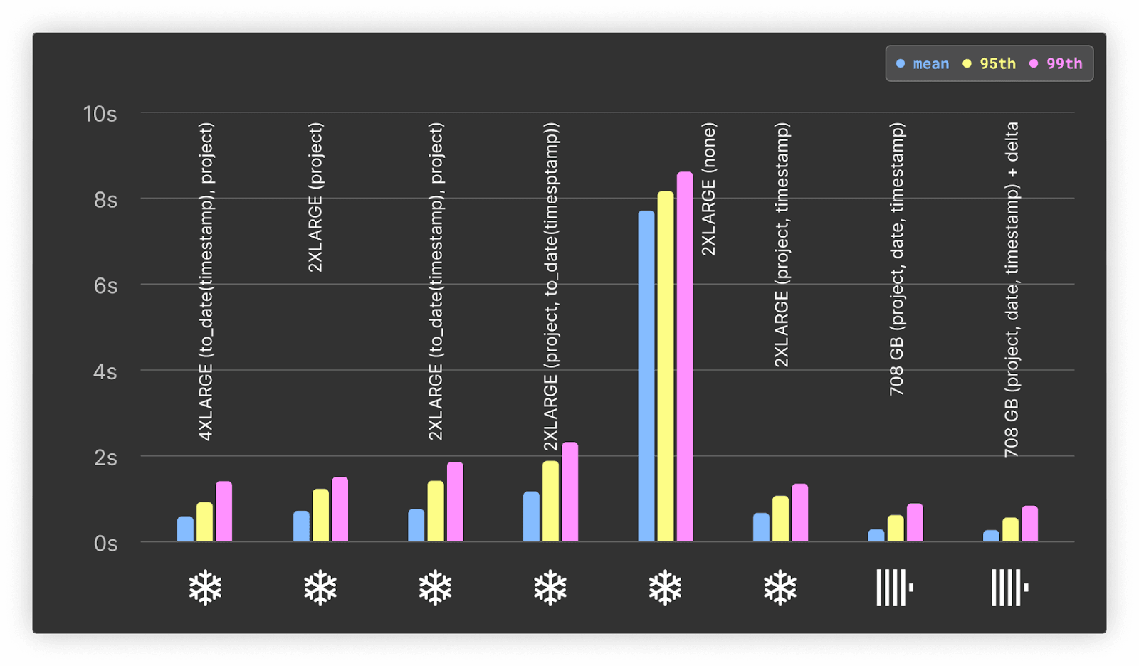
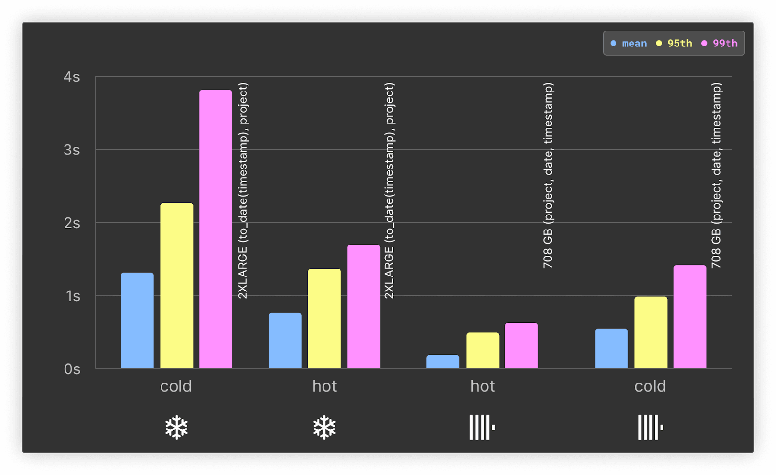
Summary of results:
- Clustering is critical to Snowflake's performance for real-time analytics, with an average response time of over 7s for non-clustered performance.
- For clusters with comparable resources, ClickHouse outperforms Snowflake by at least 3x on the mean and 2x on the 95th and 99th percentile.
- ClickHouse, with 177 vCPUs, even outperforms a 4X-LARGE Snowflake warehouse with 1024 vCPUs. This suggests our specific workload gains no benefit from further parallelization, as described by Snowflake.
Query 2: Downloads per day by Python version
This query aims to test the rendering and filtering of a multi-series line chart (by a clustered/primary key) showing downloads for a project over time. The queries aggregate downloads by day for the last 90 days, grouping by minor Python version (e.g. 3.6) and filtering by the project. A narrower time filter is then applied to a random time frame (same random values for both databases) to simulate a user drill-down. By default, this uses the 100 most popular projects for a total of 200 queries. Note that here we still filter by columns in the ordering/clustering keys but aggregate on an arbitrary low cardinality column.
SELECT
    date AS day,
    concat(splitByChar('.', python)[1], '.', splitByChar('.', python)[2]) AS major,
    count() AS count
FROM pypi
WHERE (python != '') AND (project = 'boto3') AND (date >= (CAST('2023-06-23', 'Date') - toIntervalDay(90)))
GROUP BY
    day,
    major
ORDER BY
    day ASC,
    major ASC
The full results, queries and observations can be found here.
In these tests, we used the clustering key to_date(timestamp), project for Snowflake. This performs well when considering compression, hot and cold performance, and response time on both the initial and drill-down queries.
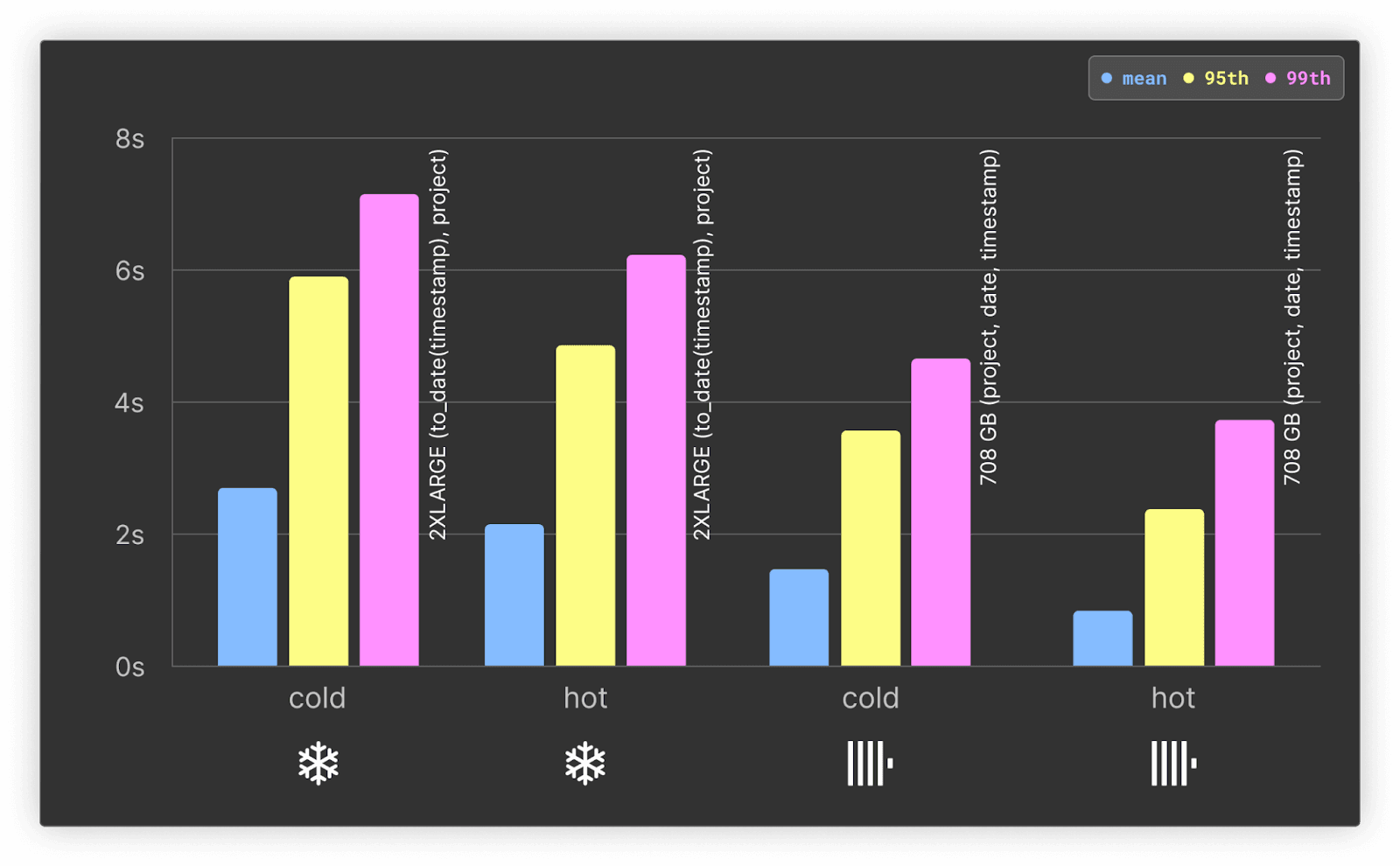
For both hot and cold queries, ClickHouse is at least 2x faster than Snowflake.
Query 3: Downloads per day by system
This query tests the rendering and filtering of a multi-series line chart showing systems for a project over time. In this case, while we filter by columns in the ordering and clustering configuration, we aggregate by a different column. This column is similar to the previous test, but the system column has a much higher cardinality. This test first aggregates downloads by day for the last 90 days, grouping by system and filtering by project. The higher cardinality of the system column requires us to filter by the top 10 values for each project to avoid excessive results. This is achieved through a sub-query that obtains the top 10 system for the project and is a realistic approach when rendering a multi-series line chart for a high cardinality column. A narrower time filter is then applied to a random time frame (same random values for both databases).
SELECT
    date AS day,
    system.name AS system,
    count() AS count
FROM pypi
WHERE (project = 'boto3') AND (date >= (CAST('2023-06-23', 'Date') - toIntervalDay(90))) AND (system IN (
    -- sub query reading top 10 systems for the project
    SELECT system.name AS system
    FROM pypi
    WHERE (system != '') AND (project = 'boto3')
    GROUP BY system
    ORDER BY count() DESC
    LIMIT 10
))
GROUP BY
    day,
    system
ORDER BY
    day ASC,
    count DESC
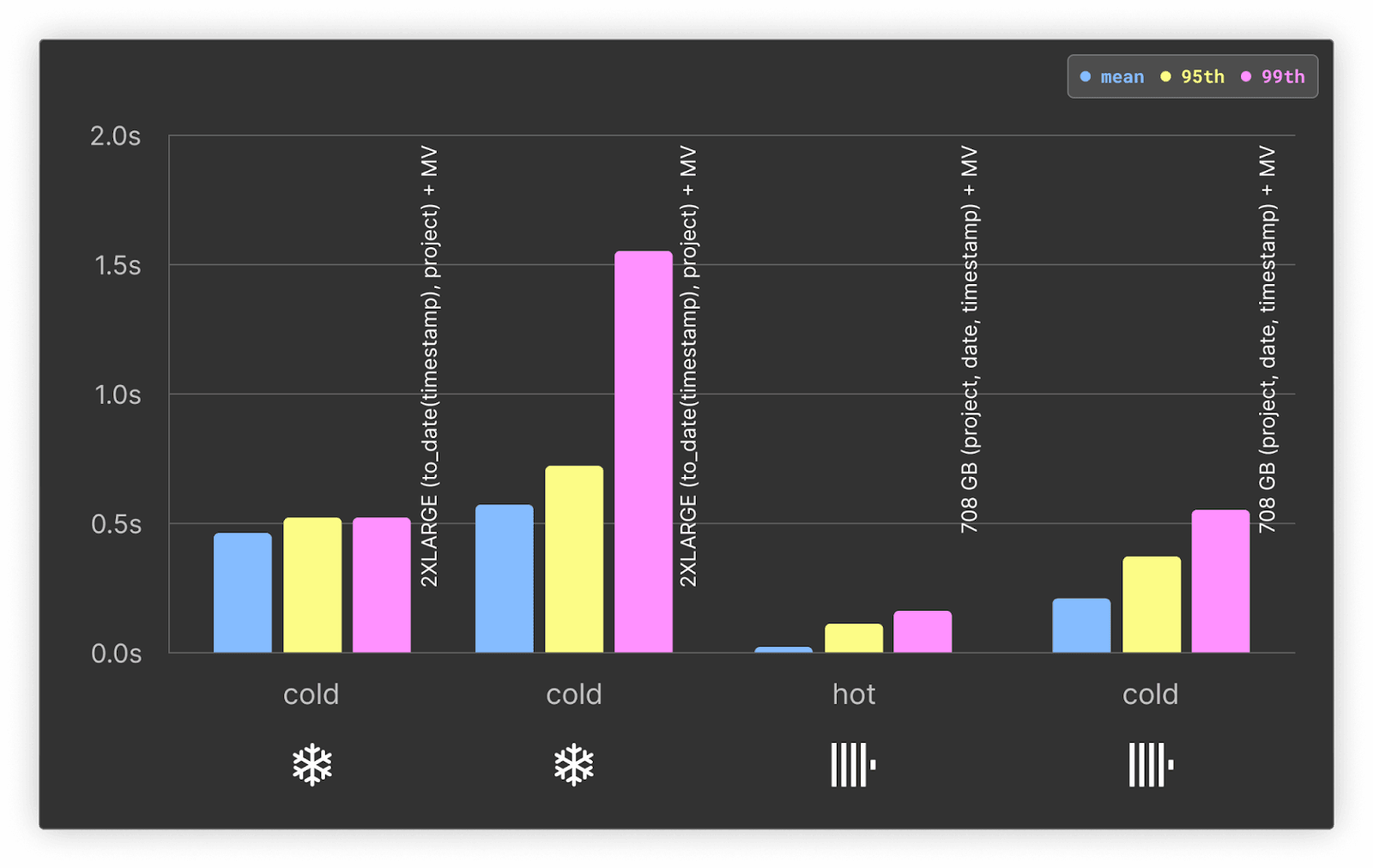
This sub-query here allows us to compare projections and their equivalent feature in Snowflake: materialized views.
The full results, queries and observations can be found here.
Hot only
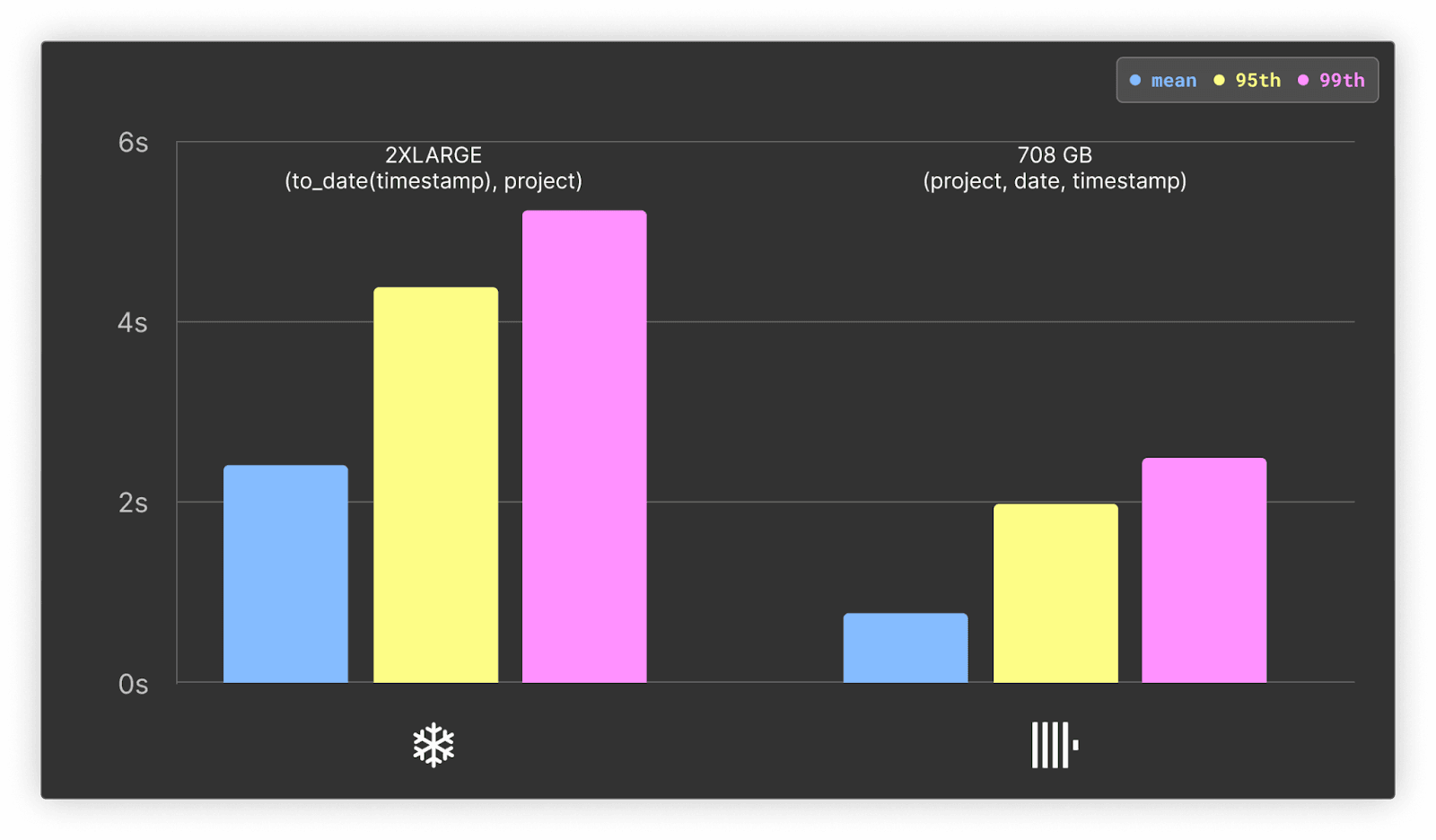
ClickHouse is at least 2x faster across all metrics for this query.
ClickHouse also outperforms Snowflake on cold queries by atleast 1.5x on the mean.
ClickHouse also outperforms Snowflake on all but the max time for cold queries, with the mean being 1.7x faster. Results here.
As mentioned above, the subquery identifying the top systems for a project is an ideal candidate to optimize with a projection in ClickHouse and materialized view in Snowflake (with clustering).
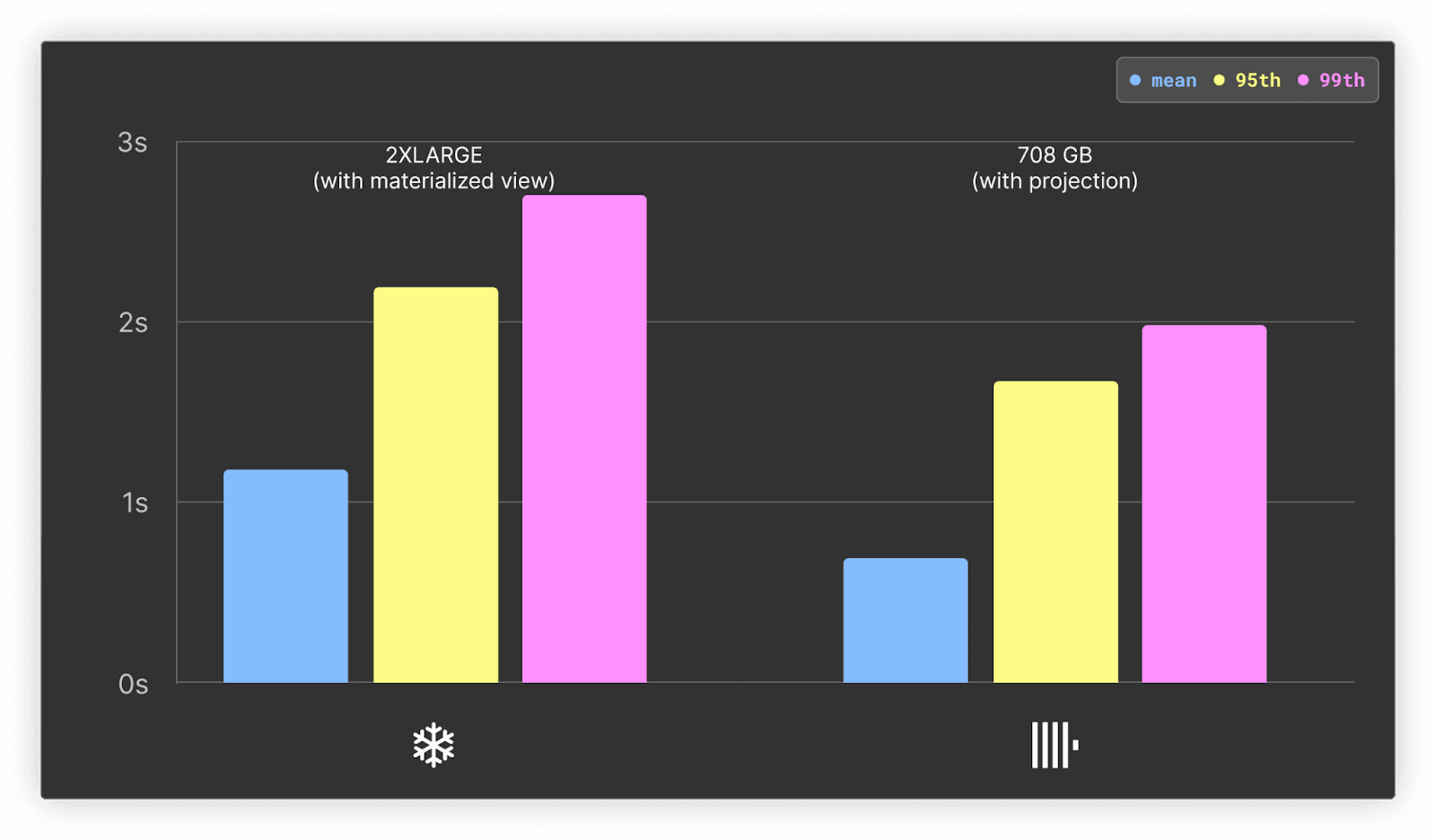
For ClickHouse, this optimization improves the mean by only 10%, but significantly impacts the 95th and 99th percentile by reducing them by 15% and 20%, respectively. While Snowflake experiences an approximately 50% improvement across metrics, ClickHouse is still around 1.5x faster.
Users deploying materialized views in Snowflake should be aware they can result in significant additional costs. In addition to requiring an enterprise plan, which raises the cost per credit to $3, they require a background service to maintain. These costs cannot be predicted and require experimentation. ClickHouse Cloud does not charge separately for projections or materialized views, although users should test the impact on insert performance, which will depend on the query used.
Query 4: Top file type per project
This query simulates the rendering and filtering of a pie chart showing file types for a project. After aggregating by file type for the last 90 days for a specific project, a narrower time filter is then applied to a random time frame. Unlike previous queries, this time filter is rounded to a day granularity, so that we can exploit materialized views in ClickHouse and Snowflake for the parent query, i.e. we can group by day instead of seconds (this would be equivalent to the main table).
SELECT
    file.type,
    count() AS c
FROM pypi
WHERE (project = 'boto3') AND (date >= (CAST('2023-06-23', 'Date') - toIntervalDay(90)))
GROUP BY file.type
ORDER BY c DESC
LIMIT 10
The full results, queries and observations can be found here.
ClickHouse is at least 2x faster on both hot and cold queries. ClickHouse and Snowflake are also approximately twice as fast for their respective hot queries than the cold. Both systems benefit from time filters being rounded to the nearest day, with mean performance faster than previous tests.
Since our drill-down queries round to the nearest day, these queries can be easily converted to materialized views in both technologies. While these are not equivalent features in Snowflake and ClickHouse, they can both be used to store summarized versions of the data, which will be updated at insert time. Full details on applying this optimization can be found here.
Materialized views have a considerable impact on performance of this query:
In ClickHouse, the materialized view improves the performance of cold queries by 2x, and of hot queries by greater than 4x - even high percentiles run in low milliseconds as a result. Conversely, Snowflake performance improves by a similar amount for cold and hot queries - 2x to 2x. This leads to a bigger gap in query performance between ClickHouse and Snowflake, with the former at least 3x faster.
Query 5: Top projects by distro
This query simulates building a pie chart where filtering is performed using a non-primary key (distro.name). This aggregates on a project, counting the number of downloads over the last 90 days, where a filter is applied to distro.name. For this, we use the top 25 distros. For each distro, we issue a subsequent query with a filter applying to a random time range (same for both databases).
The focus here is performance when filtering by a non-clustered or ordered column. This is not a complete linear scan, as we are still filtering by date/timestamp, but we expected performance to be much slower. These queries will therefore benefit from distributing computation across all nodes in the cluster. In Snowflake, this is performed by default. In ClickHouse Cloud, the same can be achieved by using parallel replicas. This feature allows the work for an aggregation query to be spread across all nodes in the cluster, reading from the same shard. This feature, while experimental, is already in use for some workloads in ClickHouse Cloud, and is expected to be generally available soon.
SELECT
    project,
    count() AS c
FROM pypi
WHERE (distro.name = 'Ubuntu') AND (date >= (CAST('2023-06-23', 'Date') - toIntervalDay(90)))
GROUP BY project
ORDER BY c DESC
LIMIT 10
The full results, queries and observations can be found here.
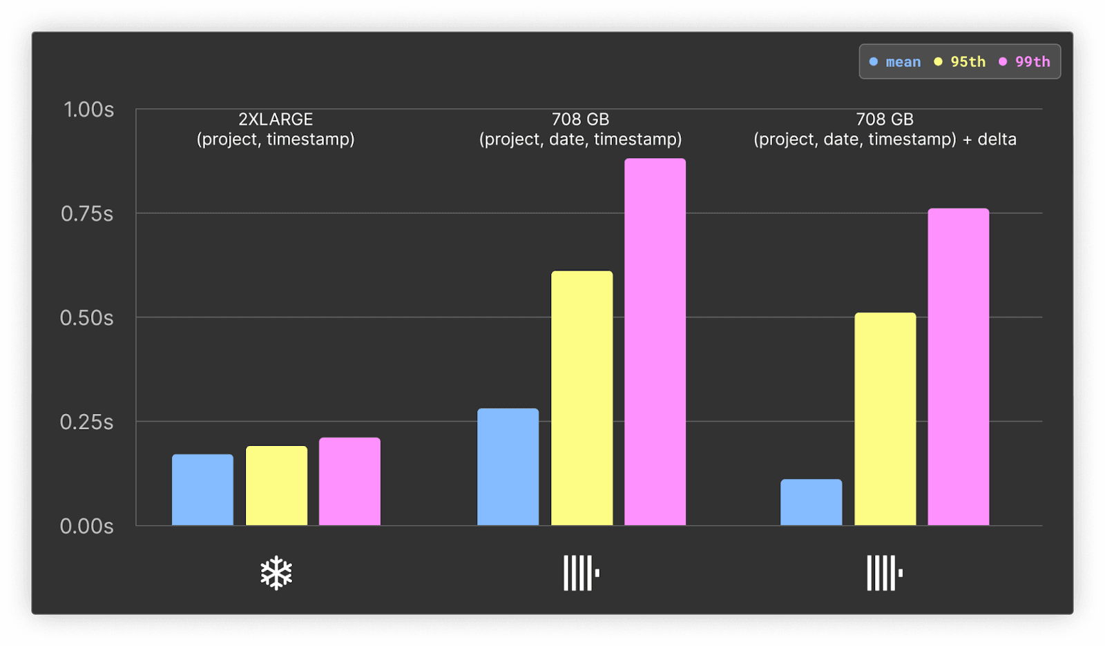
Below, we show the performance benefit of enabling parallel replicas for ClickHouse using the original 708GB service and ordering key of project, date, timestamp. This service contains a total of 177 vCPUs spread over 3 vCPUs.
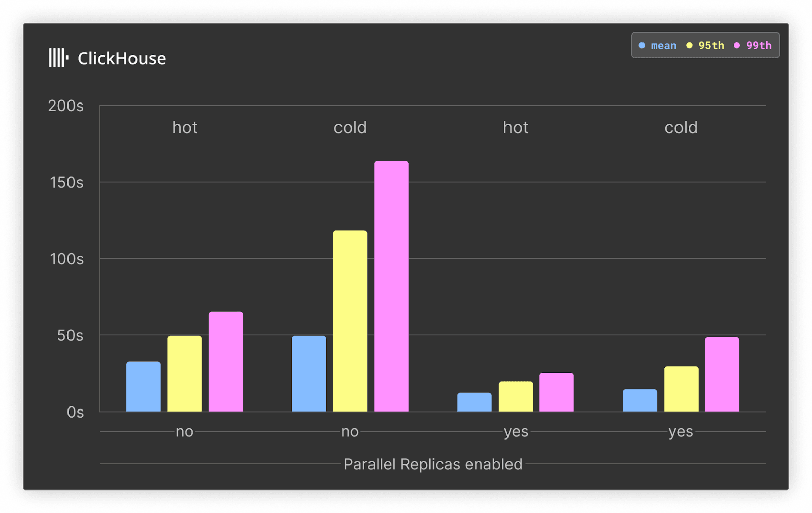
In both the hot and cold cases, ClickHouse Cloud query times are around 3x faster with parallel replicas. This is expected since all three nodes are used for the aggregation. This shows the power of parallel replicas for queries where more data needs to be scanned.
In our previous queries, the date and timestamp columns were the 2nd and 3rd entries in our ClickHouse ordering key, respectively (with project 1st) - unlike Snowflake, where it was beneficial to have the date first. In this workload, we have no project filter. We thus optimize this workload using a date, timestamp ordering key in ClickHouse to align with Snowflake.
Results for ClickHouse and Snowflake:
For ClickHouse, the best performance is achieved using the largest 1024GB service with 256 vCPUs (the same approximate vCPUs as the Snowflake 2X-LARGE warehouse).
For these queries, Snowflake is faster by around 30%. This can be attributed to the experimental nature of the parallel replicas feature, with it undergoing active development to improve performance. At the time of writing, however, Snowflake performs well on queries that can be distributed to many nodes and are required to scan significant volumes of data.
Query 6: Top sub-projects
This query tests the rendering and filtering of a pie chart showing sub-projects over time. Sub-projects are those that are related to core technology, e.g. mysql. These are identified by using project ILIKE %<term>%, where <term> is selected from a list. This list is identified by taking the top 20 prefixes of names with - in their name. For example:
SELECT splitByChar('-', project)[1] as base
from pypi
GROUP BY base
ORDER BY count() DESC
LIMIT 20
This test aggregates sub-projects for the last 90 days, sorting by the number of downloads and filtering to a project term. A narrower time filter is then applied to a random time frame, simulating a user viewing top sub-projects for a term over a time period and then drilling down to a specific time frame.
This query, while filtering on the project column, cannot fully exploit the primary key due to the use of the LIKE operator, e.g. `project LIKE '%clickhouse%". An example ClickHouse query:
SELECT
    project,
    count() AS c
FROM pypi
WHERE (project LIKE '%google%') AND (date >= (CAST('2023-06-23', 'Date') - toIntervalDay(90)))
GROUP BY project
ORDER BY c DESC
LIMIT 10
This provides an opportunity to utilize Snowflake's Search Optimization Service, which can be used to improve LIKE queries. We contrast this with ClickHouse various secondary indices which can be used to speed up such queries. Those work as skip indices that filter data without reading actual columns. More specifically, to illustrate this functionality in this case, we use the n-grams bloom filter index for the project column.
The full results, queries and observations can be found here.
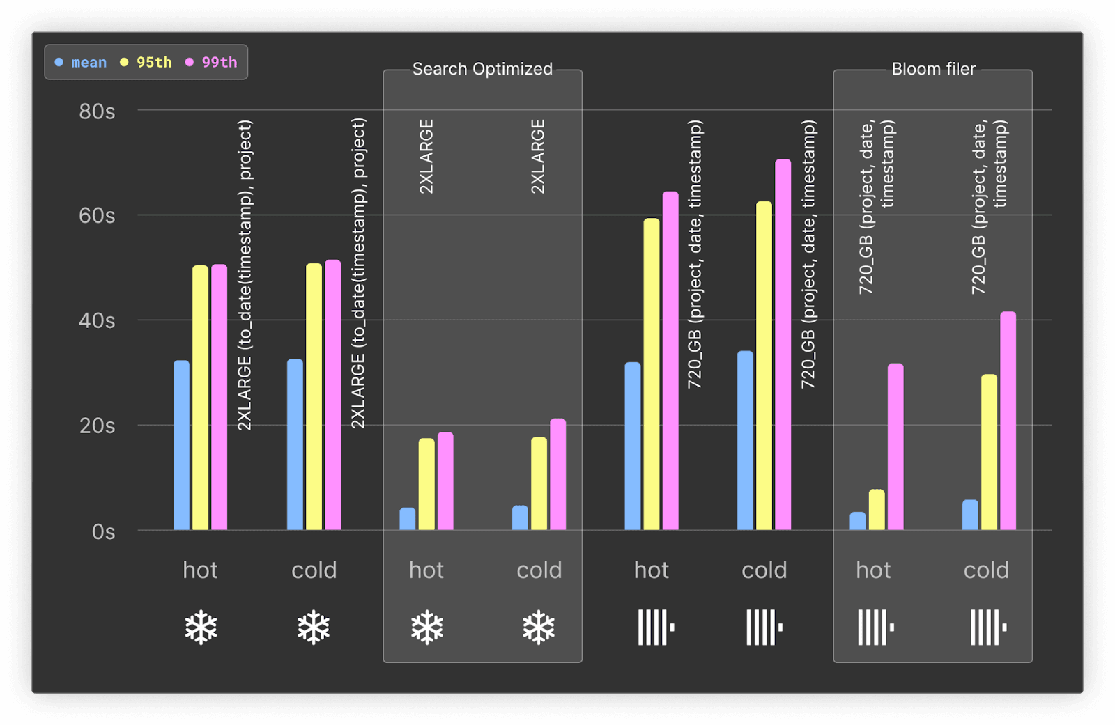
Our tests indicate the bloom filters only add 81.75MiB to our ClickHouse total storage size (compressed). Even uncompressed, the overhead is minimal at 7.61GiB.
Without the bloom filter, Snowflake and ClickHouse perform similarly for the LIKE queries - with Snowflake even outperforming ClickHouse on the 95th and 99th percentile by up to 30%.
ClickHouse bloom filters improve performance for the mean by almost 10x, and higher percentiles by at least 2x for both hot and cold queries.
Bloom filters result in ClickHouse comfortably outperforming Snowflake across all metrics with at minimum 1.5x the performance and 9x for the average case. The bloom filter also incurs no additional charges beyond a minimal increase in storage.
The Search Optimization Service significantly improves Snowflake’s performance. While still slower on average than ClickHouse for hot queries, when using the bloom filter, it is faster for cold queries and 99th percentiles. As noted in our cost analysis, however, this comes at a significant cost that makes it almost not viable to use.
Query 7: Downloads per day (with cache)
For previous tests, the query cache in Snowflake and ClickHouse has been disabled. This provides a more realistic indication of performance for queries in real-time analytics use cases, where either the queries are highly variable (and thus result in cache misses), or the underlying data is changing (thus invaliding the cache). Nonetheless, we have evaluated the impact of the respective query caches on performance for our initial Downloads per day query.
SELECT
    toStartOfDay(date),
    count() AS count
FROM pypi
WHERE (project = 'typing-extensions') AND (date >= (CAST('2023-06-23', 'Date') - toIntervalDay(90)))
GROUP BY date
ORDER BY date ASC
The full results, queries and observations can be found here.
Summary of results:
- While the ClickHouse query cache delivers a faster mean response time, Snowflake does provide a better distribution of values with lower 95th and 99th values. We attribute this to ClickHouse’s cache being local to each node and load balancing of queries. Snowflake likely benefits here from having a distributed cache at its service layer, independent of the nodes. While this may deliver a slightly high mean response time, it is more consistent in its performance. In a production scenario, changing data would invalidate these cache benefits in most real-time analytics use cases.
- For cold queries, ClickHouse benefits from higher CPU-to-memory ratios, outperforming Snowflake by 1.5 to 2x, depending on the metric.
Cost analysis
In this section, we compare the costs of ClickHouse Cloud and Snowflake. To achieve this, we calculate the cost of running our benchmarks, considering data loading, storage, and completing all queries. This analysis also highlights the additional costs incurred to make Snowflake a viable solution to real-time analytics and competitive in performance with ClickHouse Cloud. Finally, we provide a simple costing for a production service using the 2 comparable service/warehouse sizes used in our testing.
Our results demonstrate that ClickHouse Cloud is more cost effective than Snowflake across every dimension. Specifically,
To run our benchmarks:
- Data loading: Snowflake is at a minimum 5x more expensive to load data than ClickHouse Cloud.
- Querying: Querying costs in Snowflake are at a minimum 7x more expensive than ClickHouse Cloud, with Snowflake queries running in tens of seconds, and ClickHouse Cloud queries returning in seconds or less. To bring Snowflake to comparable query performance, Snowflake is 15x more expensive than ClickHouse Cloud.
For a production system:
Snowflake is at a minimum 3x more expensive than ClickHouse Cloud when projecting costs of a production workload running our benchmark queries. To bring Snowflake to comparable performance to ClickHouse Cloud, Snowflake is 5x more expensive than ClickHouse Cloud for these production workloads.
Base costs
ClickHouse and Snowflake services/warehouses have the following costs per hour:
- Snowflake: 2X-LARGE - 32 credits per hour. Credit cost depends on tier. We assume the standard tier ($2 per credit) unless otherwise stated, which is $64 per hour.
- ClickHouse: 708GB, 177 core ClickHouse Service - $0.6888 per hour per 6 CPUs, $20.3196 per hour.
- ClickHouse: 960GB, 240 core ClickHouse Service - $0.6888 per hour per 6 CPUs, $27.552 per hour.
Benchmarking cost
Summary
| Database | Bulk Data Loading Cost ($) | Clustering Cost ($) | Storage Cost per month ($) | Cost of Query Benchmark* ($) |
|---|---|---|---|---|
| Snowflake Standard | 203 | 900 | 28.73 | 185.9 |
| Snowflake Enterprise | 304 | 1350 | 28.73 | 378.98 |
| ClickHouse | 41 | 0 | 42.48 | 25.79 |
* with clustering
ClickHouse Cloud was more cost effective than Snowflake for our benchmarks:
- Data loading: Snowflake is at minimum 5x more expensive to load data than ClickHouse Cloud for our benchmarks. If clustering is utilized to ensure query performance is competitive with ClickHouse, additional costs mean data loading is 25x more expensive for Snowflake.
- Querying: Querying costs in Snowflake are at a minimum 7x more expensive than ClickHouse Cloud, with Snowflake queries running in tens of seconds, and ClickHouse Cloud queries returning in seconds or less. To bring Snowflake to comparable query performance, Snowflake is 15x more expensive than ClickHouse Cloud.
Assumptions
- We have selected the warehouse and service sizes of 2X-LARGE and 708GB for Snowflake and ClickHouse respectively. These are comparable in their total number of cores and were used throughout benchmarks.
- For our real-time analytics use case, where we are providing globally-accessible Python package analytics, we assume queries are frequent. This implies that any warehouse/services will not go idle.
- Tests use Enterprise tier features for Snowflake for comparable performance to ClickHouse Cloud (materialized views or the Search Optimization Service), which increase the Snowflake cost per unit. In such cases, we have provided two alternative costs for Snowflake - Standard and Enterprise. Snowflake’s Enterprise tier also impacts the loading cost since the per unit cost is increased.
- When computing the cost of a query benchmark, we use the results for the most performant configuration (considering the tier) and compute the total time to run all of the queries, rounded to the nearest minute.
- When computing query costs, we use the total run time multiplied by the cost per minute for the service. Note that Snowflake charges per second, with a 60-second minimum each time the warehouse starts. ClickHouse Cloud performs per-minute metering. We therefore do not consider the time required for the warehouse/service to start and stop.
- For ClickHouse Cloud data load, we utilize the service which provided the fastest load time - a 960GB service and assume the user would downsize their service once load is completed.
- We assume no Cloud Services Compute charges are incurred for Snowflake. Where a more advanced feature is utilized in Snowflake, which changes the pricing tier, we adjust the per-credit price accordingly.
- When computing query costs, we have used the results where clustering is enabled. As shown in the results for
Query 1: Downloads per day, Snowflake response times are not competitive with ClickHouse without clustering and are not sufficient for real-time analytics applications. The mean response time for this workload, with no clustering key applied, is over 7.7s (2X-LARGE). This compares to 0.28s and 0.75s seconds for ClickHouse (708GB) and Snowflake respectively, when an optimal clustering key is applied. Based on this contrast, all subsequent benchmarks applied clustering to Snowflake.
Bulk data load
We assume that Snowflake warehouses and ClickHouse services are active only for the period of data load and immediately paused, once the data has been inserted. In the case of ClickHouse, we allow time for merges to reduce parts to under the recommended limit of 3000.
| Database | Specification | Number of vCPUs | Cost per hour ($) | Time for data load (seconds) | Bulk Data load cost ($) |
|---|---|---|---|---|---|
| Snowflake (standard) | 2X-LARGE | 256 | 64 | 11410 | 202 |
| Snowflake (enterprise) | 2X-LARGE | 256 | 96 | 11410 | 304 |
| ClickHouse | 708GB | 177 | 20.3196 | 10400 (174 mins) | 59 |
| ClickHouse | 960GB | 240 | 27.552 | 5391 (90 mins) | 41 |
Snowflake costs 5x more for data loading than ClickHouse Cloud for our use case.
Our approach to data load used an external stage. This incurs no charges. Users who use an internal Snowflake stage for files will incur additional charges not included here.
Clustering costs
As described above, Snowflake’s query performance was over 7 seconds without clustering enabled - this is far too slow for a real-time application. Our tests and benchmarks thus enable clustering to ensure more competitive query performance.
Clustering on the to_date(timestamp), project key consumed 450 credits. This is $900 if using the Standard tier, and $1350, if using Enterprise features. No additional cost is incurred with ClickHouse Cloud for specifying an ordering key, a comparable feature in ClickHouse.
If we consider clustering, on the Standard tier, as part of the data loading cost, Snowflake is 27x ($900 + $203 = $1103) more expensive than ClickHouse Cloud. This does not consider the ongoing charges for Snowflake clustering, which are incurred when the data is updated after inserts.
Storage
Snowflake and ClickHouse Cloud charge the following for storage in GCP us-central-1, where our benchmark was conducted. Other regions may differ, but we do not expect this to be a significant proportion of the total cost in either case. Both Snowflake and ClickHouse consider the compressed size of the data.
- ClickHouse - $47.10 per compressed TB/month
- Snowflake - $46 per compressed TB/month
Note that the above ClickHouse storage cost includes two days of backups (one every 24 hrs). For equivalent retention in Snowflake, we assume a permanent table will be used for Snowflake in production, with 1 day of time travel. This also provides seven days of failsafe support by default. Given our data is immutable and append-only, we would expect low churn in our tables and only pay the incremental cost for new data in time travel beyond the initial copy - we estimate this to be about 8% every 7 days. We have thus estimated a multiplier of 1.08 for Snowflake.
We assume the clustering/ordering keys are used in most of our benchmarks. Using these charges, we compute a total cost for the month.
| Database | ORDER BY/CLUSTER BY | Total size (TB) | Cost per TB ($) | Backup multiplier | Cost per month ($) |
|---|---|---|---|---|---|
| Snowflake | (to_date(timestamp), project) | 1.33 | 46* | 1.08 (for time travel) | $66.07 |
| ClickHouse | (project, date, timestamp) | 0.902 | 47.10 | 1 | $42.48 |
*on demand pricing
The above costing indicates that Snowflake is 1.5x more expensive for storage. However, this assumes on-demand storage pricing for Snowflake. The price per TB is reduced to $20 if storage is pre-purchased. Assuming the user is able to exploit this, the total cost for storage is estimated as $28.73.
Queries
Estimating costs in Snowflake is complex. Some of Snowflake’s fastest query performance relies on the use of non-standard features, such as materialized views and the Search Optimization Service, which are only available in the Enterprise tier. This increases the per-credit cost to $3. These services also incur additional charges, e.g. materialized views incur a background maintenance cost. Snowflake provides means of computing these, e.g. for materialized views.
To estimate the cost of queries, we have used the configuration identified as the best performing for each query type assuming a Snowflake 2X-LARGE warehouse and 708GB ClickHouse service.
For Snowflake, we therefore compute 2 pricings - Enterprise and standard. For all calculations, we use the total execution time for the fastest configuration, given the tier, and optimistically assume the warehouse is immediately paused once the test is complete. For ClickHouse timings, we round up to the nearest minute.
We do not include initial Snowflake clustering charges for the main table and assume these are incurred as part of the data load. We do, however, consider clustering charges for materialized views.
We ignore results where query caching is enabled. We assume that a production instance would be subject to changes and updates invalidating the cache. In production, we would still recommend enabling this for both databases. As the caching results are comparable, we would not expect a meaningful impact on the ratio of costs.
ClickHouse
| Test | Ordering columns | Features used | Cost per hour ($) | Total run time (secs) | Total Cost ($) |
|---|---|---|---|---|---|
| Query1: Downloads per day | project, date, timestamp | - | 20.3196 | 302 | $2.032 |
| Query 2: Downloads per day by Python version | project, date, timestamp | - | 20.3196 | 685 | $4.064 |
| Query 3: Downloads per day by system | project, date, timestamp | Materialized views | 20.3196 | 600 | $3.387 |
| Query 4: Top file type per project | project, date, timestamp | Materialized views | 20.3196 | 56 | $0.339 |
| Query 5: Top projects by distro | project, date, timestamp | - | 20.3196 | 1990 | $11.232 |
| Query 6: Top sub projects | project, date, timestamp | Bloom filters | 20.3196 | 819 | $4.741 |
| Total | 4452 | $25.79 |
Snowflake Standard
| Test | Clustering columns | Cost per credit ($) | Cost per hour ($) | Total run time (secs) | Total cost ($) |
|---|---|---|---|---|---|
| Query1: Downloads per day | date, project | 2 | 64 | 635 | $11.28 |
| Query 2: Downloads per day by Python version | date, project | 2 | 64 | 1435 | $25.51 |
| Query 3: Downloads per day by system | date, project | 2 | 64 | 1624 | $28.87 |
| Query 4: Top file type per project | date, project | 2 | 64 | 587 | $10.44 |
| Query 5: Top projects by distro | date, project | 2 | 64 | 1306 | $23.22 |
| Query 6: Top sub projects | date, project | 2 | 64 | 4870 | $86.58 |
| Total | 10457 | $185.9 |
Snowflake Enterprise
| Test | Clustering columns | Enterprise Features used | Cost per credit ($) | Cost per hour ($) | Total run time (secs) | Warehouse Cost ($) | Additional charges | Total cost ($) |
|---|---|---|---|---|---|---|---|---|
| Query1: Downloads per day | date, project | - | 2 | 64 | 635 | $11.289 | - | $11.29 |
| Query 2: Downloads per day by Python version | date, project | - | 2 | 64 | 1435 | $25.5111 | - | $25.51 |
| Query 3: Downloads per day by system | date, project | Clustering + Materialized views | 3 | 96 | 901 | $24.027 | 61.5 credits for materialized view = $184.5 5.18 credits for clustering = $15.54 | $224.07 |
| Query 4: Top file type per project | date, project | Clustering + Materialized views | 3 | 96 | 307 | $8.187 | 0.022 credits for clustering = $0.066No materialized view charges noted. | $8.25 |
| Query 5: Top projects by distro | date, project | - | 2 | 64 | 1306 | $23.218 | - | $23.22 |
| Query 6: Top sub projects | date, project | Clustering + Search Optimization Service | 3 | 96 | 684 | $18.24 | Search optimization charges - 22.8 credits = $68.4 | $86.64 |
| Total | 5268 | $378.98 |
Querying costs in Snowflake are at a minimum 7x more expensive than ClickHouse Cloud for our benchmark tests. For Snowflake query performance to be comparable to ClickHouse Cloud's, Snowflake requires Enterprise tier features, which dramatically increases Snowflake's cost to 15x more expensive than ClickHouse Cloud.
From the above, it is clear that querying costs in Snowflake can quickly snowball, if Enterprise features are used. While they nearly always appreciably improve performance, the saving in run time does not always offset the increase in per unit cost. Users are thus left trying to identify the most cost effective way to execute each query. In comparison, ClickHouse pricing is simple - there are no additional charges for features that speed up queries.
In the above scenario, we have also assumed standard Snowflake pricing is still possible for tests where Enterprise features are not required. This leads to slightly reduced costs in the Snowflake results above, but is not realistic in production, where even using one Enterprise feature to accelerate a query will immediately cause all other queries in Snowflake to increase in cost by 1.5x. Addressing this requires complex configurations and possible data duplication.
Estimating production costs
The above benchmarking costing, while useful to highlight how costs with Snowflake can quickly add up, is difficult to extrapolate to a production scenario.
For a simple pricing model, we thus make the following assumptions:
- Our warehouse and service will be running all the time, with no idle time, because it is constantly ingesting data and serving real-time queries.
- While the full dataset is almost 10x in size, we also assume that 3 months of data is sufficient for our application.
- A 2X-LARGE and 708GB warehouse/service offer sufficient performance with respect to latency for our application.
- A 2X-LARGE and 708GB warehouse/service would be able to handle the required query concurrency of a production application.
- A 2X-LARGE and 708GB warehouse/service would not be appreciably impacted by new data being added.
- For Snowflake, we assume clustering costs are not significant (a highly optimistic assumption for Snowflake) after initial load.
- We can ignore initial data load costs here, since the warehouse/services will be running all the time.
With these assumptions, our production cost thus becomes the storage cost and time to run each warehouse and service. We present two costs for this scenario for Snowflake: Standard and Enterprise. While the latter delivers response times more competitive with ClickHouse Cloud, it comes with a 1.5x cost multiplier for Snowflake.
For ClickHouse, we assume the use of materialized views and projections where possible - these add no measurable additional cost.
Finally, we also provide pricing for a 4X-LARGE Snowflake service. Users might be tempted to use this configuration with no clustering. While queries will be slower, Snowflake has demonstrated linear scalability - queries should thus be 4x faster than a 2X-LARGE with no clustering. This performance may be acceptable e.g. queries in the Downloads per day test with a mean of 7.7s on a 2X-LARGE should take less than 2s on a 4X-LARGE.
| Database | Specification | Compute Cost per hour ($) | Compute Cost per month ($) | Data Storage Cost per month ($) | Total Cost per month ($) |
|---|---|---|---|---|---|
| Snowflake (standard) | 2X-LARGE | 64 | $46,080 | $28.73 | $46,108 |
| Snowflake (Enterprise) | 2X-LARGE | 96 | $69,120 | $28.73 | $69,148 |
| Snowflake (standard) | 4X-LARGE | 256 | $184,320 | $28.73 | $184,348 |
| ClickHouse | 708GB | 20.3196 | $14,630 | $42.48 | $14,672 |
The above shows Snowflake is over 3x more expensive to run a production application than ClickHouse Cloud. For comparable performance between both systems, through Enterprise tier features, users pay 4.7x more with Snowflake compared to ClickHouse Cloud.
In reality, we would expect this difference to be much larger, since numbers above ignore additional Snowflake charges, including:
- Clustering charges as new data is added. We have ignored these charges in Snowflake to simplify pricing, but our benchmarking costs showed them to be significant. Using a 4XLARGE with no clustering is not viable and is unlikely to be competitive as shown.
- Charges to maintain materialized views in Snowflake, if used. These, especially if combined with clustering, can be substantial, as shown by our benchmarking costs.
- Data transfer costs. These can be incurred in Snowflake, depending on the regions involved. ClickHouse Cloud does not charge for data transfer costs.
- Data staging costs were not incurred in our testing, as we used an external stage and simply imported data from a GCS bucket. Internal stages do incur charges in Snowflake and may be required in some cases. ClickHouse Cloud has no concept of stages.
Real-world scenarios impose additional restrictions. After benchmarking different specifications of systems, decisions on an actual size should be made. Parameters of the given workload have direct implications during capacity planning. Those can be hard limits to process some workload during a period of time, or capacity to process a number of parallel queries with low latencies. In any case, some amount of work needs to be done over a period of time.
Below, you can see an example of how the amount of work per day differs, if we utilize 100% time of a cluster and run one benchmark at a time.
| Database | Specification | Total benchmark time (s) | Benchmark runs per day | Compute cost per day | Benchmark runs per $1k |
|---|---|---|---|---|---|
| Snowflake (standard) | 2X-LARGE | 10457 | 8.26 | 1536 | 5.37 |
| Snowflake (Enterprise) | 2X-LARGE | 5268 | 16.40 | 2304 | 7.11 |
| ClickHouse | 708GB | 4452 | 19.40 | 488 | 39.76 |
The above shows that the amount of work that can be processed by ClickHouse is 5.5x higher than Snowflake for the same compute cost. Note that, as described above, Snowflake’s costs increase dramatically with the use of query-accelerating features like materialized views and clustering.
Conclusion
This blog post has provided a comprehensive comparison of Snowflake and ClickHouse Cloud for real-time analytics, demonstrating that for a realistic application, ClickHouse Cloud outperforms Snowflake in terms of both cost and performance for our benchmarks:
- ClickHouse Cloud is 3-5x more cost-effective than Snowflake in production.
- ClickHouse Cloud querying speeds are over 2x faster compared to Snowflake.
- ClickHouse Cloud results in 38% better data compression than Snowflake.
Contact us today to learn more about real-time analytics with ClickHouse Cloud. Or, get started with ClickHouse Cloud and receive $300 in credits.