This post demonstrates how data in ClickHouse can be used to train models through a feature store. As part of this, we also show how the common tasks that data scientists and engineers need to perform when exploring a dataset and preparing features can be achieved in seconds with ClickHouse over potentially petabyte datasets with SQL. To assist with feature creation, we use the open-source feature store Featureform, for which ClickHouse was recently integrated.
We initially provide a quick recap of why users might want to use ClickHouse for training machine models and how a feature store helps with this process. Users familiar with these concepts can skip straight to the examples below.
This post will be the first in a series where we train models with Featureform, gradually building a more complex machine-learning platform with a suite of tools to take our model to production. In this initial post, we demonstrate the building blocks using feature stores to help train Logistic Regression and Decision Tree-based classifiers with data in ClickHouse.
Feature ≈ Column
We use the term "feature" throughout this post. As a reminder, a feature is some property of an entity that has predictive power for a Machine Learning (ML) model. An entity, in this sense, is a collection of features as well as a class or label representing a real-world concept. The features should, if of sufficient quality and if such a relationship exists, be helpful in predicting the entity's class. For example, a bank transaction could be considered an entity. This may contain features such as the amount transacted and purchase/seller involved, with the class describing whether the transaction was fraudulent.
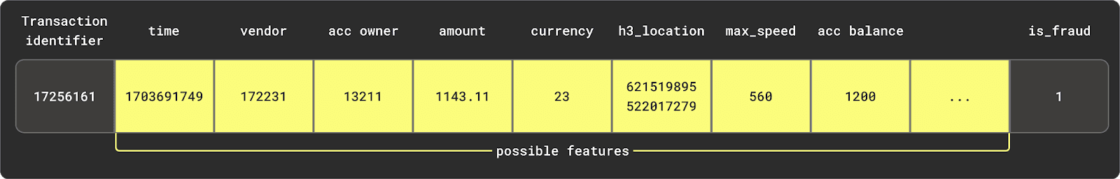
In the case of structured data, we can consider a feature to be a column - from either a table or result set. We use the terms interchangeably here, but it's worth remembering that features usually require some prior data engineering steps and data transformation logic before they are available for use.
Feature stores
We recently published a blog post describing the different types of feature stores, why you may need one, and their main components. As part of this, we explored how these are used to train machine learning models. Below, we do a short recap for those new to this concept.
In summary, a feature store is a centralized hub for storing, processing, and accessing commonly used features for model training, inference, and evaluation. This abstraction provides convenience features such as versioning, access management, and automatically translating the definition of features to SQL statements.
The main value here is improving collaboration and reusability of features, which in turn reduces model iteration time. By abstracting the complexity of data engineering from data scientists and only exposing versioned high-quality features through an API, model reliability and quality may be improved.
A feature store consists of a number of key components. In this blog, we focus on two: the transformation engine and the offline store.
Prior to any model being trained, data must first be analyzed to understand its characteristics, distributions, and relationships. This process of evaluation and understanding becomes an iterative one, resulting in a series of ad-hoc queries that often aggregate and compute metrics across the dataset. Data scientists performing this task demand query responsiveness in order to iterate quickly (along with other factors such as cost-efficiency and accuracy). Raw data is rarely clean and well-formed and thus must be transformed prior to being used to train models. All of these tasks require a transformation and query engine that can ideally scale and is not memory-bound.
The offline store holds features resulting from the transformations, serving them to models during training. These features are typically grouped as entities and associated with a label (the target prediction). Usually, models need to consume these features selectively, either iteratively or through aggregations, potentially multiple times and in random order. Models often require more than one feature, requiring features to be grouped together in a "feature group" - usually by an entity ID and time dimension. This requires the offline store to be able to deliver the correct version of a feature and label for a specific point in time. This "point-in-time correctness" is often fundamental to models, which need to be trained incrementally.
ClickHouse as a transformation engine and offline store
While ClickHouse is a natural source of data for machine learning models (e.g., click traffic), it is also well suited to the role of a transformation engine and offline store. This offers several distinct advantages over other approaches.
As a real-time data warehouse that is optimized for aggregations and capable of scaling to petabyte datasets, ClickHouse allows users to perform transformations using the familiar language of SQL. Rather than needing to stream the data from an existing database into computational frameworks, such as Spark, data can be stored in ClickHouse, with any explorative and transformation work handled at the source.
ClickHouse pre-built statistical and aggregation functions make this SQL easy to write and maintain. Fundamentally, this architecture benefits from data locality, delivering unrivaled performance and allowing billions of rows to be distilled down to several thousand with aggregation queries.
The results of these transformations can also persist in ClickHouse via INSERT INTO SELECT statements or simply be exposed as views. With transformations often grouped by an entity ID and returning a number of columns as results, ClickHouse’s schema inference can automatically detect the required types from these results and produce an appropriate table schema to store them.
These resulting tables and views can then form the base of an offline store, serving data to model training.
Features are effectively extracted and expressed as SQL queries returning tabular data.
In summary, by using ClickHouse as both the transformation engine and offline store, users benefit from data locality and the ability of ClickHouse to parallelize and execute computationally expensive tasks across a cluster. This allows the offline store to scale to PBs, leaving the feature store to act as a lightweight coordination layer and API through which data is accessed and shared.
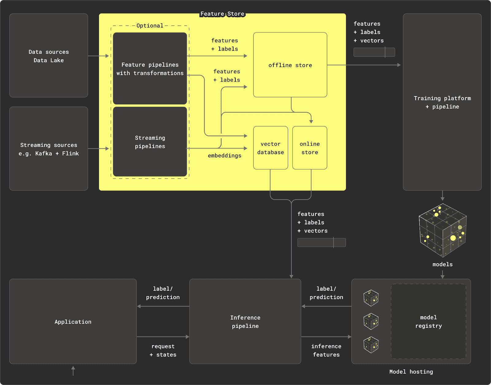
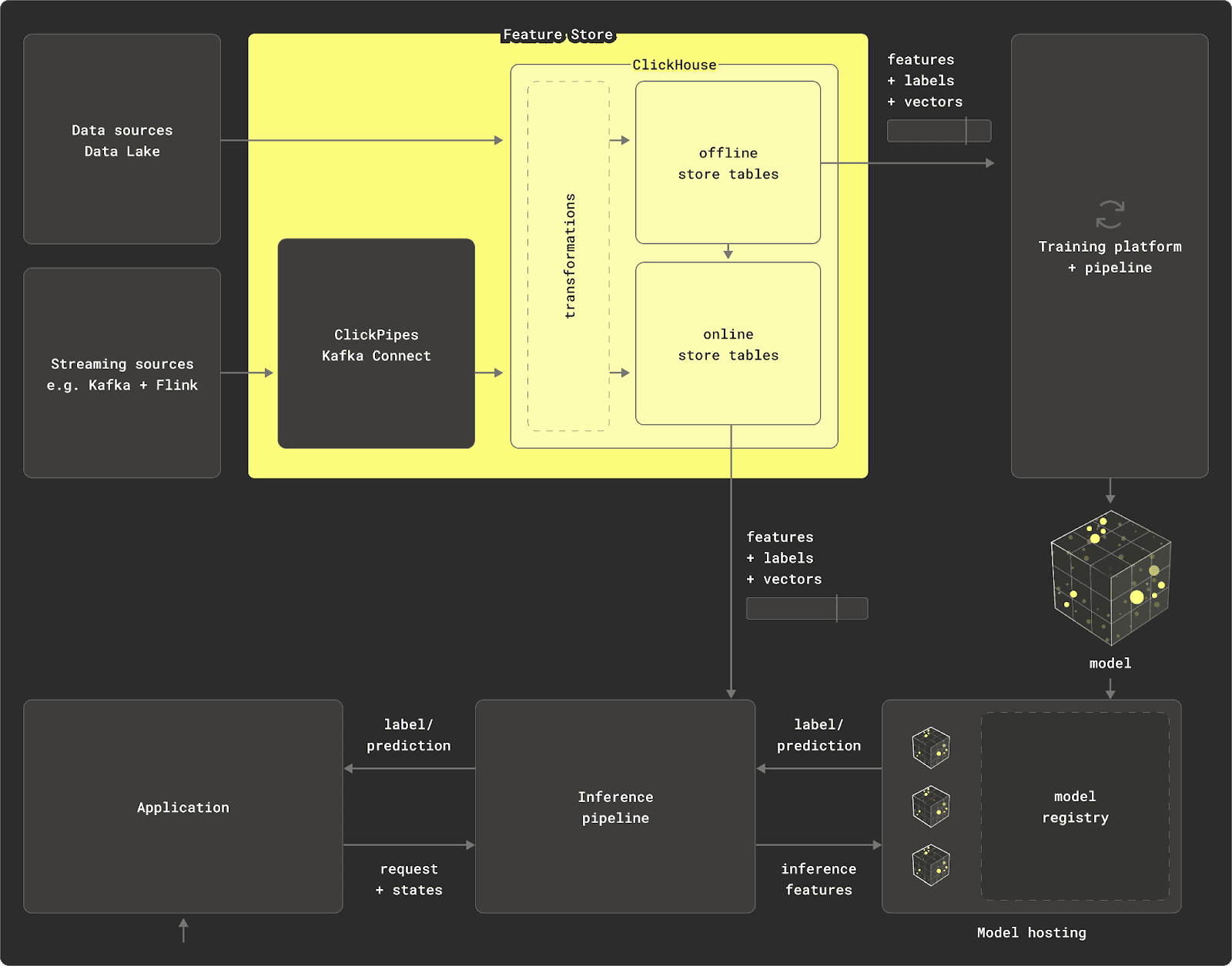
These diagrams highlight additional key components of a feature store, notably the online store. Once a model is trained, it's deployed for real-time predictions, requiring both immediate data, like a user's ID, and precomputed features, such as historical purchases, which are too costly to generate on-the-fly. These features, stored in the online store for quick access, are crucial for latency-sensitive tasks like fraud detection. They are updated from the offline store to ensure they reflect the latest data. For more information, see our earlier blog post. While ClickHouse can be used as an online store, in this post we focus on the training examples and thus on the roles of transformation engine and offline store.
Featureform
Our previous post explored different types of feature stores: Physical, Literal, and Virtual. The Virtual store is best suited to ClickHouse, providing it with the opportunity to be used as both the offline store and transformation engine. In this architecture, the feature store is not responsible for managing transformations and the persistence and versioning of features but acts as an orchestrator only.
To realize our vision of a virtual feature store, super-charged by ClickHouse, we identified Featureform as an ideal solution with which to integrate. As well as being open-source, allowing us to easily contribute, Featureform also offers mature (by design) integration points for offline stores, online stores, and vector databases.
Getting started with Featureform and ClickHouse
First we install featureform with a simple pip installation:
pip install featureformWhile Featureform employs a modular architecture that can be deployed in Kubernetes, for our initial example, we’ll use the excellent getting started experience. In this mode, all components of the architecture are deployed as a single docker container. Even better, a simple flag ensures that ClickHouse is deployed with a test dataset preloaded.
(.venv) clickhouse@PY test_project % featureform deploy docker --quickstart --include_clickhouse
DeprecationWarning: pkg_resources is deprecated as an API. See https://setuptools.pypa.io/en/latest/pkg_resources.html
Deploying Featureform on Docker
Starting Docker deployment on Darwin 23.3.0
Checking if featureform container exists...
    Container featureform not found. Creating new container...
    'featureform' container started
Checking if quickstart-postgres container exists...
    Container quickstart-postgres not found. Creating new container...
    'quickstart-postgres' container started
Checking if quickstart-redis container exists...
    Container quickstart-redis not found. Creating new container...
    'quickstart-redis' container started
Checking if quickstart-clickhouse container exists...
    Container quickstart-clickhouse not found. Creating new container...
    'quickstart-clickhouse' container started
…

Featureform is now running!
To access the dashboard, visit http://localhost:80
Run jupyter notebook in the quickstart directory to get started.
This gives us a ClickHouse, FeatureForm, Redis, and Postgres container. The latter two of these we can ignore for now.
Test dataset
At this point, we can connect to our ClickHouse container via the ClickHouse client and confirm the test dataset has been loaded.
(.venv) dalemcdiarmid@PY test_project % clickhouse client
ClickHouse client version 24.1.1.1286 (official build).
Connecting to localhost:9000 as user default.
Connected to ClickHouse server version 24.2.1.

55733a345323 :) SHOW TABLES IN fraud

SHOW TABLES FROM fraud

┌─name───────┐
│ creditcard │
└────────────┘

1 row in set. Elapsed: 0.005 sec.
For our test dataset, we use a popular fraud dataset distributed on Kaggle, consisting of over 550,000 anonymized transactions, with the objective of developing fraud detection algorithms.
A source of inspiration
Wanting to focus this blog on the mechanics of working with ClickHouse and Featureform, we looked for previous efforts that had successfully trained a model for this dataset.
Recognizing data scientists often prefer to work in Notebook environments, there are a number on Kaggle that attempt to fit models to this dataset, classifying whether a transaction is fraud or not. Attracted to the somewhat unrealistic title of "Credit Card Fraud Detection with 100% Accuracy," but impressed with the layout and methodical nature of the code, we use this as the basis of our example. Shout out to Anmol Arora for their contribution.
We acknowledge that the models used in these notebooks (Logistical Regressions/Decision Trees) do not represent the “state of the art” algorithms for classification. However, the purpose of this blog post is to show how models can be trained with ClickHouse and Featureform and not to represent the “best” or “latest” techniques possible in predicting fraud. Feel free to adapt any examples to use more modern techniques! P.s. I’m also not an ML expert.
Connecting Featureform and ClickHouse
Remember that Featureform will provide the feature store interface through which we access our data in ClickHouse, allowing us to define reusable and versioned features that we can pass to a model for training. This requires us to register our ClickHouse server with Featureform. This requires only a few lines of code, where we first define a Featureform client (local and insecure for this simple test example) before registering our local ClickHouse instance.
Note we use the environment variable
FEATUREFORM_HOSTto specify the location of the Featureform instance. These connection details can alternatively be passed to the client directly.
# install any dependencies into our notebook
!pip install featureform==1.12.6
!pip install river -U
!pip install scikit-learn -U
!pip install seaborn
!pip install googleapis-common-protos
!pip install matplotlib
!pip install matplotlib-inline
!pip install ipywidgets

%env FEATUREFORM_HOST=localhost:7878
%matplotlib inline
from featureform import Client
import featureform as ff
import matplotlib.pyplot as plt
import seaborn as sns
from sklearn.linear_model import SGDClassifier, LogisticRegression
from sklearn.metrics import classification_report
from sklearn.metrics import accuracy_score
import numpy as np

# Featureform client. Local instance and insecure
client = Client(insecure=True)
# Register our local container with Featureform
clickhouse = ff.register_clickhouse(
   name="clickhouse",
   description="A ClickHouse deployment for example",
   host="host.docker.internal",
   port=9000,
   user="default",
   password="",
   database="fraud"
)
client.apply(verbose=True)
The
client.apply()method in Featureform creates the defined resources. These are otherwise evaluated lazily and are created as required (i.e. when used downstream). Registering this dataset causes it to be internally copied in ClickHouse using anINSERT INTO SELECT, effectively making an immutable copy of the data for analysis that Featureform has versioned. See below for further details.
Registering a table
In addition to acting as a transformation engine and offline store, ClickHouse is, first and foremost, a data source in the ML Ops workflow. Before we can transform and extract features from our fraud table, we first need to register this table in Featureform. This creates the necessary metadata in Featureform so we can version and track our data. The code for this is minimal.
creditcard = clickhouse.register_table(
   name="creditcard",
   table="creditcard",
)
data = client.dataframe(creditcard, limit=100)
data.info()

<class 'pandas.core.frame.DataFrame'>
RangeIndex: 100 entries, 0 to 99
Data columns (total 31 columns):
 #   Column  Non-Null Count  Dtype
---  ------  --------------  -----
 0   id      100 non-null    int64
 1   V1      100 non-null    float64
 2   V2      100 non-null    float64
 3   V3      100 non-null    float64
 4   V4      100 non-null    float64
 5   V5      100 non-null    float64
 6   V6      100 non-null    float64
 7   V7      100 non-null    float64
 8   V8      100 non-null    float64
 9   V9      100 non-null    float64
 10  V10     100 non-null    float64
 11  V11     100 non-null    float64
 12  V12     100 non-null    float64
 13  V13     100 non-null    float64
 14  V14     100 non-null    float64
 15  V15     100 non-null    float64
 16  V16     100 non-null    float64
 17  V17     100 non-null    float64
 18  V18     100 non-null    float64
 19  V19     100 non-null    float64
 20  V20     100 non-null    float64
 21  V21     100 non-null    float64
 22  V22     100 non-null    float64
 23  V23     100 non-null    float64
 24  V24     100 non-null    float64
 25  V25     100 non-null    float64
 26  V26     100 non-null    float64
 27  V27     100 non-null    float64
 28  V28     100 non-null    float64
 29  Amount  100 non-null    float64
 30  Class   100 non-null    int64
dtypes: float64(29), int64(2)
memory usage: 24.3 KB
Our second line here fetches 100 rows of the underlying data as a data frame - this LIMIT is pushed down to ClickHouse, providing us with our final opportunity to see the columns we are working with.
This aligns with the description of the dataset, in which columns V1 to V28 provide anonymized features in addition to the transaction Amount. Our Class denotes whether the transaction is fraud, represented as a boolean with values 1 and 0.
Transforming data
With our dataset registered in Featureform, we can begin to use ClickHouse as a transformation engine.
For effective training of any classifier, we should understand the distribution of the classes.
While we could compute this over our previous data frame, this limits our analysis to the 100 rows it contains.
data['Class'].value_counts().plot.pie(autopct='%3.1f%%',shadow=True, legend= True,startangle =45)
plt.title('Distribution of Class',size=14)
plt.show()
Ideally, we’d like to compute this for all of the rows in the table. For our dataset, we could probably just load the entire dataset of 550k rows into memory by removing the limit. However, this is not viable for the larger datasets from either a network or memory perspective. To push this work down to ClickHouse, we can define a transformation.
@clickhouse.sql_transformation(inputs=[creditcard])
def classCounts(creditcard):
    return "SELECT Class,count() c FROM {{creditcard}} GROUP BY Class"

client.dataframe(classCounts).pivot_table(index='Class', columns=None, values='c', aggfunc='sum').plot.pie(
    explode=[0.1, 0], autopct='%3.1f%%', shadow=True, legend=True, startangle=45, subplots=True)
We use a simple aggregation here to compute the count per class. Note the use of templating for our query. The variable {{creditcard}} will be replaced with the table name of the credit card dataset. This will not be the original table - as we noted earlier, with Featureform making an immutable copy of the data in ClickHouse, this will be a table with a name specific to the version. Once created, we can convert the results of the transformation into a data frame and plot the results.
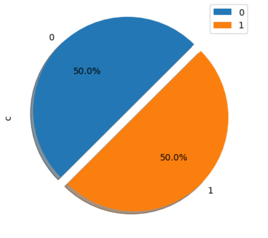
This dataset is balanced (50% fraud and 50% non fraud). While this significantly simplifies future training, it makes us wonder if this dataset is artificial. This is also likely to heavily contribute to the rather high accuracy scores advertised in the original notebook.
With our primary data serving as the raw materials, these are then transformed into data sets containing the set of features and labels required for serving and training machine learning models. These transformations can be directly applied to primary data sets or sequenced and executed on other previously transformed data sets. It’s essential to understand that Featureform does not perform the data transformations itself. Instead, it orchestrates ClickHouse to execute the transformation. The results of the transformation will also be stored as a versioned table in ClickHouse for later fast retrieval - a process known as materialization.
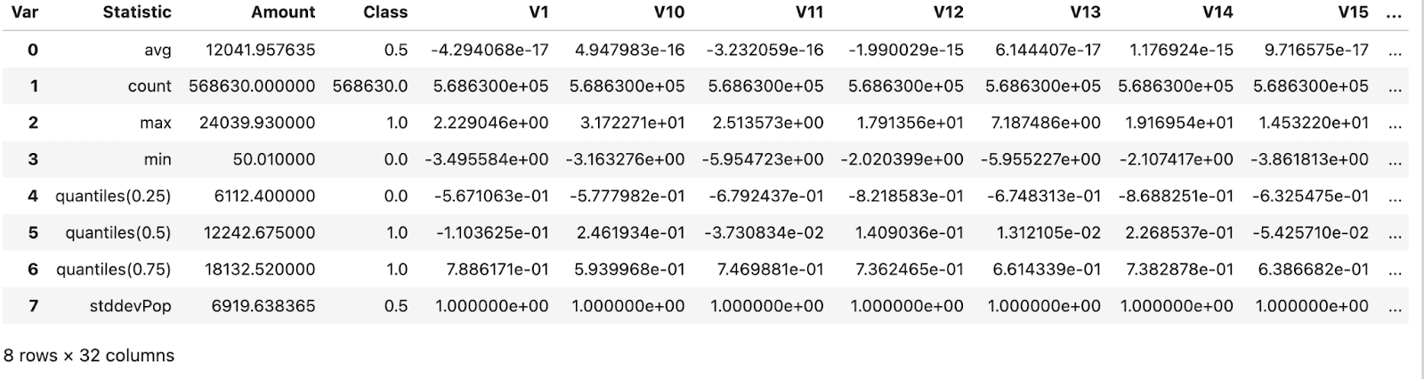
Similarly, when first exploring data, users often use the describe method for a data frame to understand the properties of the columns.
data.describe()
This requires us to compute several statistics for every column in the dataset. Unfortunately, the SQL query for this is quite complex as it exploits dynamic column selection.
import re
@clickhouse.sql_transformation(inputs=[creditcard])
def describe_creditcard(creditcard):
    return "SELECT * APPLY count, * APPLY avg, * APPLY std, * APPLY x -> (quantiles(0.25)(x)[1]), * APPLY x -> (quantiles(0.5)(x)[1]), * APPLY x -> (quantiles(0.75)(x)[1]), * APPLY min, * APPLY max FROM {{creditcard}}"

df = client.dataframe(describe_creditcard, limit=1)
df_melted = df.melt()
df_melted['Var'] = df_melted['variable'].apply(lambda x: re.search(r"\((\w*)\)", x).group(1))
df_melted['Statistic'] = df_melted['variable'].apply(
    lambda x: re.search(r"(.*)\(\w*\)", x).group(1).replace('arrayElement(', ''))
df_melted.pivot(index='Statistic', columns='Var', values='value').reset_index()
In later versions of the Featureform integration, we would like to abstract this complexity away from the user. Ideally,
describe()should formulate the required ClickHouse query for the user and execute this transparently for the user. Stay tuned.
Our final notebook, which users can find in the Featureform example repository, contains a number of transformations designed to perform an analysis of the data. These reproduce the work done by the author of the original notebook, which used pandas directly. We highlight a few of the more interesting transformations below.
Correlation matrices can help us understand any linear relationships between variables/columns in our dataset. In pandas, this requires a corr method call on the data frame. This specific operation is quite computationally expensive on very large datasets. In SQL, this requires the use of the ClickHouse corrMatrix function. The following transformation pivots the results to be consistent with the format expected by the popular Seaborn visualization library.
@clickhouse.sql_transformation(inputs=[creditcard])
def credit_correlation_matrix(creditcard):
    return """WITH matrix AS
    (
        SELECT arrayJoin(arrayMap(row -> arrayMap(col -> round(col, 3), row),
               corrMatrix(id, V1, V2, V3, V4, V5, V6, V7, V8, V9, V10, V11, V12, V13, V14,
               V15, V16, V17, V18, V19, V20, V21, V22, V23, V24, V25, V26, V27, V28, Amount, Class))) AS matrix
        FROM {{creditcard}}
    )
    SELECT
        matrix[1] AS id, matrix[2] AS V1, matrix[3] AS V2,  matrix[4] AS V3, matrix[5] AS V4,
        matrix[6] AS V5,  matrix[7] AS V6, matrix[8] AS V7, matrix[9] AS V8, matrix[10] AS V9,
        matrix[11] AS V10, matrix[12] AS V11, matrix[13] AS V12, matrix[14] AS V13,
        matrix[15] AS V14, matrix[16] AS V15, matrix[17] AS V16, matrix[18] AS V17,
        matrix[19] AS V18, matrix[20] AS V19, matrix[21] AS V20,  matrix[22] AS V21,
        matrix[23] AS V22, matrix[24] AS V23, matrix[25] AS V24, matrix[26] AS V25,
        matrix[27] AS V26, matrix[28] AS V27, matrix[29] AS V28, matrix[30] AS Amount,
        matrix[31] AS Class
    FROM matrix"""

client.dataframe(credit_correlation_matrix)
paper = plt.figure(figsize=[20, 10])
sns.heatmap(client.dataframe(credit_correlation_matrix, limit=100), cmap='crest', annot=True)
plt.show()
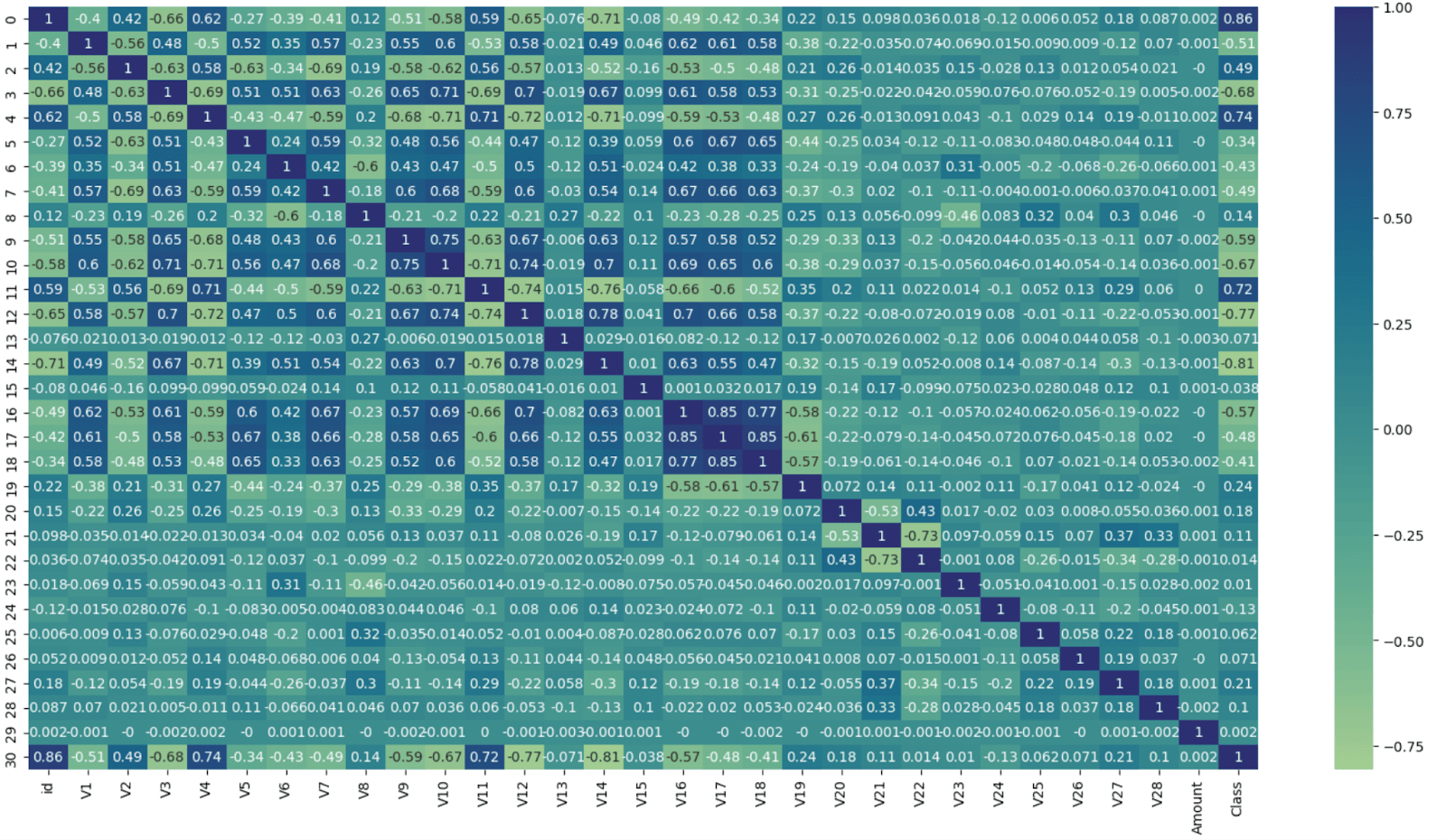
From this, we can make the same observations as the original notebook, namely that a few of our features/columns are highly correlated.
- V17 and V18
- V16 and V17
- V16 and V18
- V14 has a negative correlation with V4
- V12 is also negatively correlated with V10 and V11.
- V11 is negatively correlated with V10 and positively with V4.
- V3 is positively correlated with V10 and V12.
- V9 and V10 are also positively correlated.
- Several features show a strong correlation with the target class variable.
Logistic regression assumes that there is no perfect multicollinearity among the independent variables. We may, therefore, want to drop some features and their associated column which are strongly correlated before training.
Typically, we might use the results here to identify redundant features. A high correlation between two features suggests that they might convey similar information, and one can potentially be removed without losing significant predictive power. Additionally, correlation with the target variable can highlight which features are most relevant. However, the original notebook obtained good results without doing this.
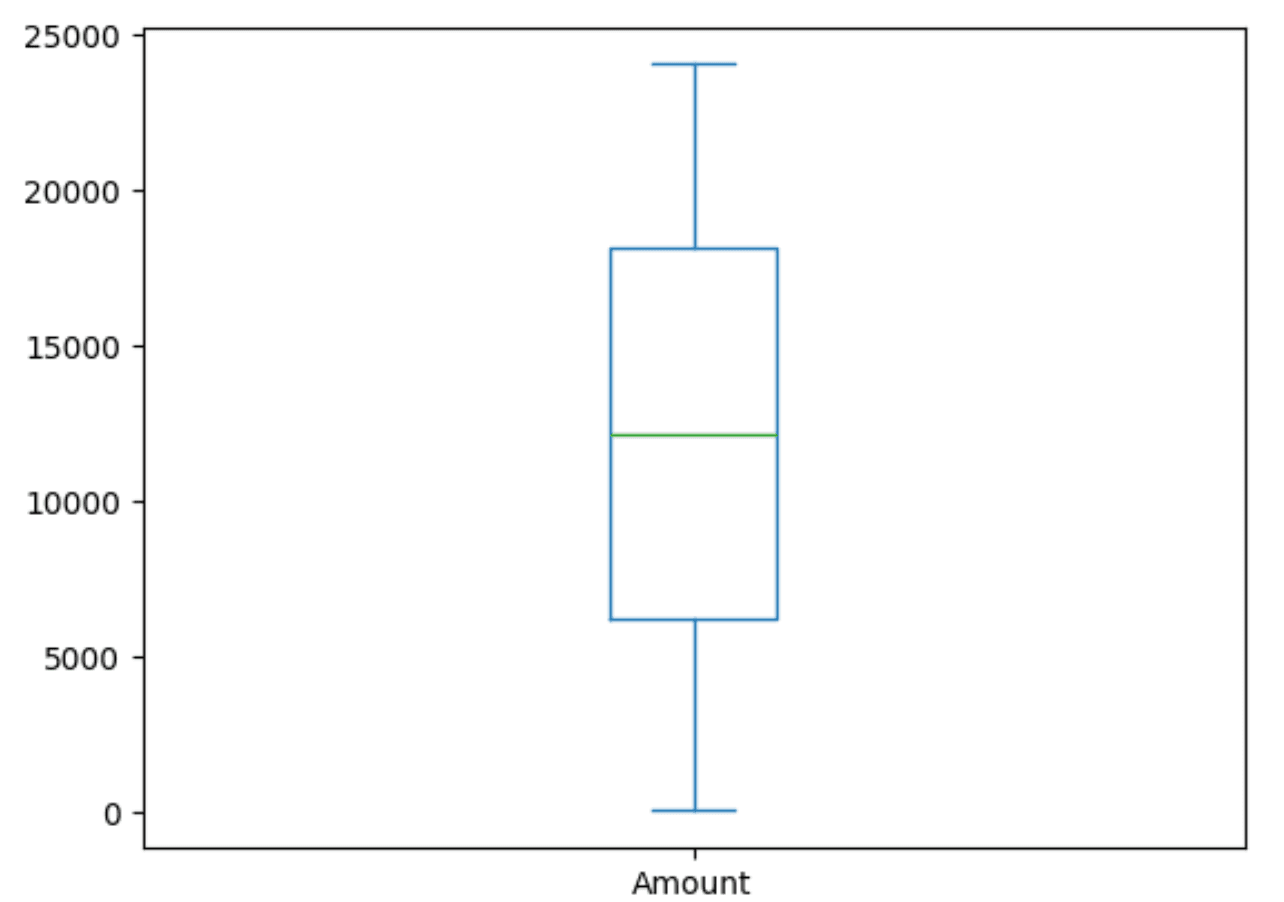
While most of our V* features are in the same range, we can see from our earlier .describe() that Amount has a different scale. We can confirm this scale with a simple box plot.
@clickhouse.sql_transformation(inputs=[creditcard])
def amountQuantitles(creditcard):
    return "SELECT arrayJoin(quantiles(0, 0.25, 0.5, 0.75, 1.)(Amount)) AS Amount FROM {{creditcard}}"
client.dataframe(amountQuantitles).plot.box()
This confirms we will need to apply a scalar to these values prior to using them in any regression model.
While decision trees can handle missing values, logistic regression techniques cannot inherently handle missing data directly in the model-fitting process. While there are techniques for handling this, we should confirm if this is required beforehand. Additionally, it's helpful to identify duplicates. Both of these can be handed with two simple transformations.
@clickhouse.sql_transformation(inputs=[creditcard])
def anynull_creditcard(creditcard):
    return "SELECT * APPLY x -> sum(if(x IS NULL, 1, 0)) FROM {{creditcard}}"

client.dataframe(anynull_creditcard, limit=1).melt()

@clickhouse.sql_transformation(inputs=[creditcard])
def credit_duplicates(creditcard):
    return "SELECT *, count() AS cnt FROM {{creditcard}} GROUP BY * HAVING cnt > 1"

client.dataframe(credit_duplicates, limit=1)
We don’t include the results here (lots of boring 0s and empty tables!), but our data has no duplicates or missing values.
Scaling values
Scaling features is an important step prior to attempting to train a logistic regression model, which uses a gradient descent algorithm to optimize the model's cost function. When features are on different scales, the imbalance can lead to slow convergence because the learning algorithm makes smaller steps in some directions and larger steps in others, potentially oscillating or taking a prolonged path to reach the minimum.
The original notebook scaled the dataset using the StandardScalar, available in Scikit Learn, for all the columns. We replicate this using another transformation.
@clickhouse.sql_transformation(inputs=[creditcard])
def scaled_credit_cards(creditcard):
    column_averages = ', '.join([f'avg(V{i})' for i in range(1, 29)])
    column_std_deviations = ', '.join([f'stddevPop(V{i})' for i in range(1, 29)])
    columns_scaled = ', '.join(f'(V{i} - avgs[{i}]) / stds[{i}] AS V{i}' for i in range(1,29))
    return f"WITH ( SELECT [{column_averages}, avg(Amount)] FROM {{{{creditcard}}}} ) AS avgs, (SELECT [{column_std_deviations}, stddevPop(Amount)] FROM {{{{creditcard}}}}) AS stds SELECT id, { columns_scaled }, (Amount - avgs[29])/stds[29] AS Amount, Class FROM {{{{creditcard}}}}"

client.apply()
Here, we calculate the average and std deviation of each column before computing and returning the column value - avg/std.deviation - thus replicating a StandardScalar operation.
The results of this transformation represent a version of the data stored as a table in ClickHouse that we can use for our model training.
Model training
With our data scaled, we can train our first model. One of the benefits of using ClickHouse as your training source is its ability to aggregate and transform data quickly. Featureform materializes these transformations, storing them as a new table for fast iteration and reuse. While our transformation here has been very simple - a simple scalar function, it could equally be a GROUP BY over several trillion rows to return a result set of several thousand.
In this role, ClickHouse now acts as an offline store to serve the data.
As a first step, we need to define an entity. This entity consists of a set of features and a class, per our earlier description. In Featureform, this is simple:
@ff.entity
class Transaction:
    # Register multiple columns from a dataset as features
    transaction_features = ff.MultiFeature(
        scaled_credit_cards,
        client.dataframe(scaled_credit_cards, limit=10),
        include_columns=[f"V{i}" for i in range(1, 29)] + ["Amount"],
        entity_column="id",
        exclude_columns=["Class"],
    )
    fraud = ff.Label(
        scaled_credit_cards[["id", "Class"]], type=ff.Bool,
    )
Note how we need to specify an entity identifier (the id column) and use our previously created transformation scaled_credit_cards as the source. We exclude the Class from our features, as you might expect, given it's our target Label, and specify this accordingly.
With an entity defined, we can register a training set. The terminology here can be a little confusing as this will contain both our training and testing set. We’ll skip using a validation set for now since we aren’t doing any hyperparameter tuning or trying to identify an optimal algorithm.
fraud_training_set = ff.register_training_set(
    "fraud_training_set",
    label=Transaction.fraud,
    features=Transaction.transaction_features,
)
client.apply()
As always, our resources are lazily evaluated, so we explicitly call apply. This causes our training set to be created, again as a versioned table in ClickHouse that is only exposed through the Featureform API.
Under the hood, each feature is represented by its own table. This allows new entities to be composed of features. This might not be necessary in our simple example, but it unlocks collaboration and reusability, as we’ll discuss later.
With our "training set" ready, we now need to split this into a training and validation set. For Featureform, this is a simple call, requiring us to specify the ratio of the split. For this, we use a classic 80/20 split.
# fetch the training set through the FF client
ds = client.training_set(fraud_training_set)
# split our training set ino a train and test set
train, test = ds.train_test_split(test_size=0.2, train_size=0.8, shuffle=True, random_state=3, batch_size=1000)
The shuffle ensures ClickHouse delivers the data in random order (useful given our approach to training below). We also specify a random_state as a seed to this randomization, such that if we invoke the notebook multiple times, the data is delivered in the same random order.
At this point, we could simply load train into a data frame in memory and use this to train a model. To show how datasets larger than local memory can be handled, we demonstrate an iterative approach to consuming the data.
This requires us to diverge from the original notebook and use an incremental approach to training - specifically, we use a Stochastic Gradient Descent (SGD) algorithm with a log_loss function to train a Logistic regression model.
clf = SGDClassifier(loss='log_loss')
for features, label in train:
    clf.partial_fit(features, label, classes=[True,False])
Our Featureform train dataset can be efficiently iterated, delivering us batches of the previously defined size of 1000. These are used to partially and incrementally fit our regression model.
Once trained (this can take a few seconds, depending on resources), we can exploit our test dataset to evaluate our model. For brevity, we’ll skip evaluating performance against our training set.
from sklearn.metrics import confusion_matrix
def model_eval(actual, predicted):
    acc_score = accuracy_score(actual, predicted)
    conf_matrix = confusion_matrix(actual, predicted)
    clas_rep = classification_report(actual, predicted)
    print('Model Accuracy is: ', round(acc_score, 2))
    print(conf_matrix)
    print(clas_rep)

def plot_confusion_matrix(cm, classes=None, title='Confusion matrix'):
    """Plots a confusion matrix."""
    if classes is not None:
        sns.heatmap(cm, xticklabels=classes, yticklabels=classes, vmin=0., vmax=1., annot=True)
    else:
        sns.heatmap(cm, vmin=0., vmax=1.)
    plt.title(title)
    plt.ylabel('True label')
    plt.xlabel('Predicted label')

# Make a test prediction
pred_test= np.array([])
label_test = np.array([])
for features, label in test:
    batch_pred = np.array(clf.predict(features))
    pred_test = np.concatenate([pred_test, batch_pred])
    label_test = np.concatenate([label_test, np.array(label)])
model_eval(label_test, pred_test)
cm = confusion_matrix(label_test, pred_test)
plot_confusion_matrix(cm, classes=[True, False], title='')
The methods defined here simply provide us with a model accuracy metric and plot our confusion matrix. Note how we make predictions in batches, using an iterator on test, and collect these before computing accuracy and plotting a confusion matrix.
Model Accuracy is:  0.96
[[55024  1825]
 [ 2358 54519]]
              precision    recall  f1-score   support

         0.0       0.96      0.97      0.96     56849
         1.0       0.97      0.96      0.96     56877

    accuracy                           0.96    113726
   macro avg       0.96      0.96      0.96    113726
weighted avg       0.96      0.96      0.96    113726
With no tuning, the results here are impressive, with an accuracy of 96%. The original notebook takes this further, training a decision tree and random forest classifier before finally using an xgboost approach. Given the random forest delivers the best performance here, claiming 100% accuracy on both the test and training set, we thought we’d attempt to reproduce this with an incremental approach.
Continuing our approach of using an online learning method, we use a Hoeffding Adaptive Tree classifier via the River Library. This algorithm is based on the Hoeffding Adaptive Tree algorithm, a form of decision tree, which uses the Hoeffding bound to decide the minimum number of samples needed to split a node with high confidence, ensuring that the chosen split is close to the best possible split that could be made given infinite data. This method allows the tree to grow and adapt to changing data distributions as data is streamed. As data flows, the algorithm continuously evaluates the performance of its splits (nodes) and can adapt by replacing poorly performing branches with new ones.
Training this model using the Featureform APIs is very similar to our earlier SGD example.
from river import tree
from river import metrics

ds = client.training_set(fraud_training_set)
train, test = ds.train_test_split(test_size=0.2, train_size=0.8, shuffle=True, random_state=3, batch_size=1000)

# Initialize the HoeffdingAdaptiveTreeClassifier
model = tree.HoeffdingAdaptiveTreeClassifier()
# we need to pivot into [({"feature1": value1, "feature2": value2}, label), ...] for the model
feature_names = [t.name for t in Transaction.transaction_features]
n = 0
for features, label in train:
    # Update the model with the current instance
    for i, feature in enumerate(features):
        feature_dict = dict(zip(feature_names, feature))
        model.learn_one(feature_dict, label[i])
        n += 1
    print(f'{n} processed')
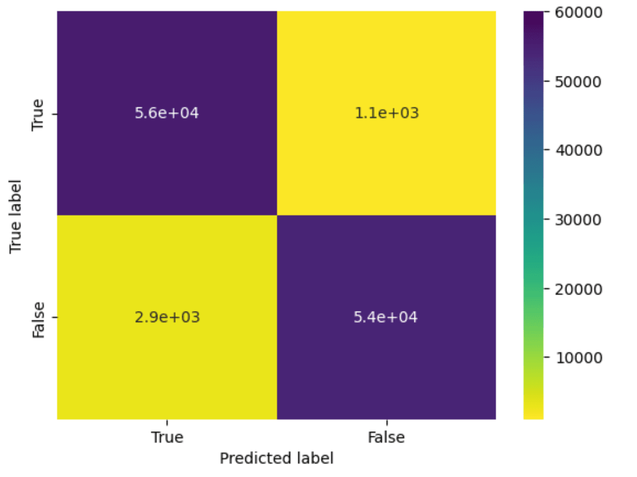
This model takes about 10 minutes to train from our Macbook 2023. Once trained, we can evaluate the model performance:
predicted_labels = []
actual_labels = []

for features, label in test:
    for i, feature in enumerate(features):
        feature_dict = dict(zip(feature_names, feature))
        predicted_labels.append(model.predict_one(feature_dict))
        actual_labels.append(label[i])

# Evaluate the model
model_eval(actual_labels, predicted_labels)

# Plot the confusion matrix
cm = confusion_matrix(actual_labels, predicted_labels)
plot_confusion_matrix(cm)
Model Accuracy is:  0.98
[[55715  1067]
 [ 1234 55710]]
              precision    recall  f1-score   support

           0       0.98      0.98      0.98     56782
           1       0.98      0.98      0.98     56944

    accuracy                           0.98    113726
   macro avg       0.98      0.98      0.98    113726
weighted avg       0.98      0.98      0.98    113726
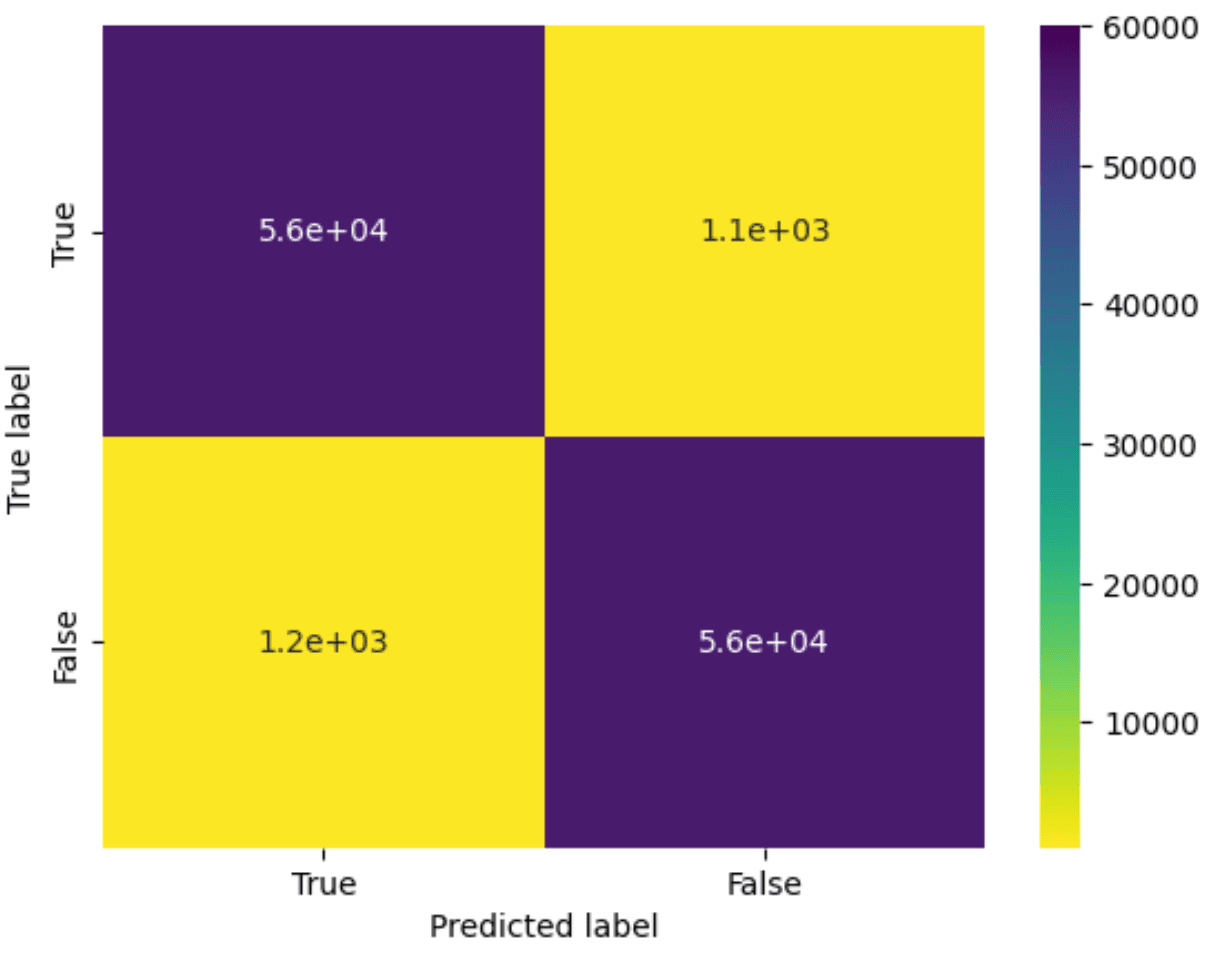
So, the quality may not be quite 100%, but we’ve managed to get comparable performance to the original notebook with an online technique. This is an over-simplistic approach to the problem, and we have definitely benefited from the data being cleaned (or artificially generated?). We would probably also prefer a model that placed an emphasis on minimizing false negatives (around 1k out of 500k in the above confusion matrix). We leave further model refinement as an exercise to the user and would welcome a critique of our efforts!
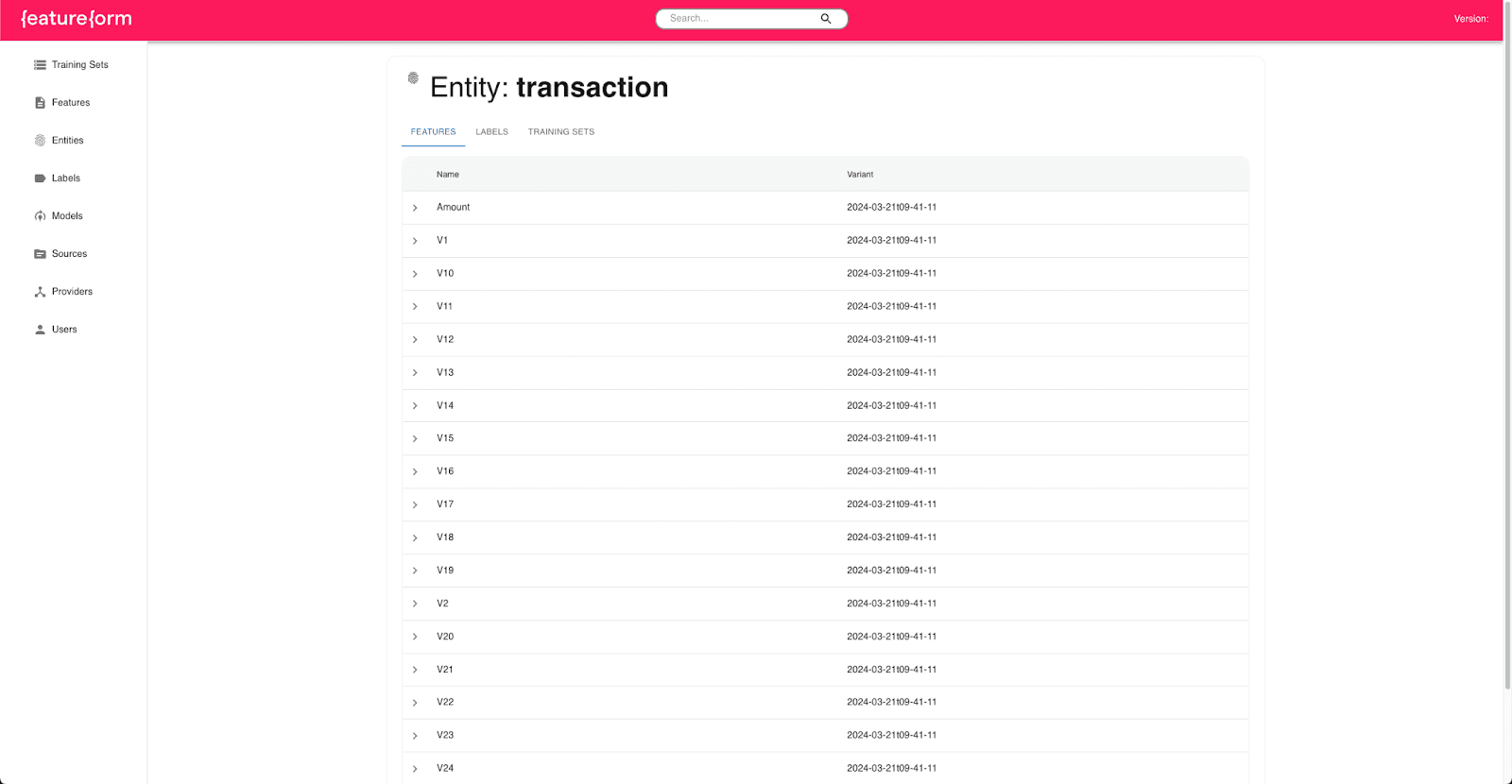
Sharing and versioning
All of the above may seem like any other notebook with a simple abstraction over ClickHouse. However, under the hood, Featureform manages the creation of state and versioning. This current state can be viewed through the user interface (http://localhost), which shows the current features, entities, labels, and training sets tracked in the system.
This state is robust to notebook restarts (it's persisted in a local database by Featureform) but, more importantly, allows these objects to be used by other data scientists and data engineers. The above features, for example, could be used by another engineer to compose a different entity, which itself could, in turn, be shared. All of this is enabled through the above Python API, which serves these objects and enables collaboration.
If you wish to explore Featureform more, we recommend familiarizing yourself with the abstractions it provides. We have also only explored where features and entities are materialized in ClickHouse as tables (or views). Featureform offers a number of other features, including on-demand features and streaming capabilities, when batch processing is not appropriate.
Throughout this blog, we've mentioned how objects in Featureform are versioned without explicitly showing how. Featureform uses a mechanism known as variants to version data sources, transformations, features, labels, and training sets. Each of these resources is immutable by default, ensuring you can confidently utilize versioned resources created by others without the risk of disruption due to upstream modifications.
For each resource, a variant parameter exists that can be configured either manually or automatically. Recognizing that later variants of features are not necessarily improvements over previous ones (Machine Learning isn't a linear journey of improvement, unfortunately), the term "variant" is preferred over "version". In our examples, we've simply relied on automatic versioning. If we changed any resource in our flow (e.g., change the features used for our entity), this would create a new variant of the resource and trigger the recreation of all dependency resources. This tracking of lineage requires Directed Acyclic Graphs (DAG) and employs techniques similar to tools such as dbt that users may be familiar with.
Conclusion
In this post, we've explored how ClickHouse can be used as a feature store to train machine learning models using Featureform. In this role, ClickHouse acts as both a transformation engine and an offline store. We have transformed and scaled a fraud dataset using only SQL and used the subsequent data to incrementally train both Logistic regression and Decision tree-based models to predict whether transactions are fraudulent or not. In the process, we have commented on how using an SQL database with feature stores allows a collaborative approach to feature engineering, improving the usability of features, which in turn reduces model iteration time. In future posts, we will explore how we can take this model to production and integrate with tooling such as AWS Sagemaker for model training.