
Introduction
PostgreSQL and ClickHouse represent the best of class concerning open-source databases, each addressing different use cases with their respective strengths and weaknesses. Having recently enabled our PostgreSQL (and MySQL) integrations in ClickHouse Cloud, we thought we’d take the opportunity to remind users of how these powerful integrations can be used with ClickHouse. While we focus on Postgres, all functions have their equivalent MySQL versions and should be easily derived.
In the first part of this series, we look at the PostgreSQL function and table engine. A second post will explore the database engine and demonstrate how Postgres can be used in conjunction with ClickHouse dictionaries.
If you want to dive deeper into these examples, ClickHouse Cloud is a great starting point - spin up a cluster using a free trial, load the data, let us deal with the infrastructure, and get querying!
Interested in trying the Postgres integration in ClickHouse Cloud? Get started instantly with $300 free credit for 30 days.
We use a development service in ClickHouse Cloud – a production service could be used, either is fine. For our Postgres instance, we utilize Supabase which offers a generous free tier sufficient for our examples.
Supabase offers significantly more than just a Postgres database and is a full Firebase alternative with Authentication, instant APIs, Edge Functions, Realtime subscriptions, and Storage. If you want to build a real application using the data in this post, Supabase will accelerate its development and deployment.
Complementary
PostgreSQL, also known as Postgres, is a free and open-source relational database management system focused on extensibility, SQL compliance, and ACID properties via transactions. As the world’s most popular OSS OLTP (Online transaction processing) database , it is used for use cases where data is highly transactional and there is a need to support thousands of concurrent users.
ClickHouse is an open-source column-oriented OLAP (Online analytical processing) database for real-time analytical workloads. With a focus on supporting lightning-fast analytical queries, it typically serves use cases such as real-time analytics, observability, and data warehousing.
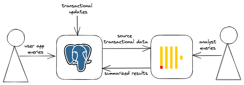
A successful architectural pattern using ClickHouse in conjunction with PostgreSQL to power an analytics “speed layer” has recently emerged. In this paradigm, PostgreSQL is used as the transactional source of truth and serves the operational use case where row-based operations are dominant. Advanced analytical queries, however, are better served via ClickHouse leveraging its column-oriented model to answer complex aggregates on the millisecond scale. This complementarity relationship benefits greatly from the tight integration that exists between the two OSS technologies.
The business case & dataset
Scenario: we are running a property listing website serving thousands of users. Prices can be updated and/or rows deleted as properties are delisted or reduced in price. This represents a great use case for Postgres, which will hold our source of truth for the data. Our imaginary business would also like to perform analytics on this data, creating a need to move data between Postgres and ClickHouse.
For our examples, we use relatively small instances of Postgres and ClickHouse: the developer tier in ClickHouse Cloud (Up to 1 TB storage and 16 GB total memory) and the free tier in Supabase. The latter limits the database size to 500 MB. Therefore, we have selected a dataset of moderate size that fits our business use case and these instance sizes: the UK house price dataset. Used throughout our documentation, this largely fits these requirements with only 28m rows. Each row represents a house sale in the UK in the last 20 yrs, with fields representing the price, date, and location. A full description of the fields can be found here.
We distribute this dataset as Postgres-compatible SQL, ready for insert, downloadable from here.
Loading the data
Once you’ve signed up to Supabase, create a new project under the free tier with an appropriately secure password and grab the database endpoint from the settings.
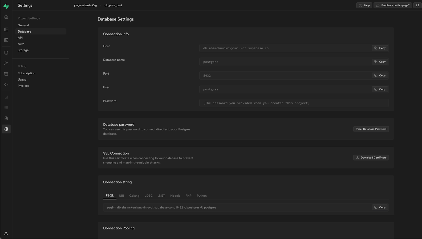
For our examples, we execute all our queries using the psql client. Supabase also offers a web client for those seeking a life away from the terminal. Our Postgres schema is shown below. We also create a few indexes which our subsequent queries should intuitively be able to utilize.
CREATE TABLE uk_price_paid
(
   id integer primary key generated always as identity,
   price INTEGER,
   date Date,
   postcode1 varchar(8),
   postcode2 varchar(3),
   type varchar(13),
   is_new SMALLINT,
   duration varchar(9),
   addr1 varchar(100),
   addr2 varchar(100),
   street varchar(60),
   locality varchar(35),
   town varchar(35),
   district varchar(40),
   county varchar(35)
)

psql -c "CREATE INDEX ON uk_price_paid (type)"
psql -c "CREATE INDEX ON uk_price_paid (town)"
psql -c "CREATE INDEX ON uk_price_paid (extract(year from date))"
Some basic analytical queries
Before loading our data in ClickHouse, let's remind ourselves why we might need our analytical workloads outside of Postgres. Note the timings of the following queries. The results presented are the fastest of five executions. We have also attempted to optimize these to exploit the indexes where possible but welcome further suggestions!
Average price per year for flats in the UK
psql -c "\timing" -c "SELECT
	extract(year from date) as year,
	round(avg(price)) AS price
FROM uk_price_paid
WHERE type = 'flat'
GROUP BY year
ORDER BY year"

 year | price
------+--------
 1995 |  59004
 1996 |  63913
…
 2021 | 310626
 2022 | 298977
(28 rows)

Time: 28535.465 ms (00:28.535)
This is slower than expected. The EXPLAIN for this query, indicates that the type index is not utilized, resulting in a full table scan. The reason for this is query planner relies on tables statistics. The cardinality of the type column is very low - 5 values, meaning 6.3M rows have a flat value out of 34M ~1/6th of the total dataset. Because type='flat' rows are distributed in all data blocks (around 24 rows per block), the probability of having flat value in any single block is very high (it’s 1/6th with 24 rows per block). The query planner therefore determines a parallel sequential scan will be more efficient than reading the index (and then searching for relevant rows in the data).
My colleague Vadim Punski actually proposed a way to speed up this query considerably. We’ve posted the solution here but excluded as it represents a rather poor use of Postgres and will result in a large storage footprint. The changes to the table schema will also not complete on Supabase’s free tier due to the 120s query timeout.
Most expensive postcodes in a city
From our above query we know that Postgres won’t use indexes if a linear scan is cheaper, due to a filter clause value existing in most blocks. If we filter by a less common city e.g. Bristol, the index can be exploited and the query performance improvement is dramatic.
psql -c "\timing" -c "SELECT
      postcode1,
      round(avg(price)) AS price
FROM uk_price_paid WHERE town='BRISTOL'
GROUP BY postcode1
ORDER BY price DESC LIMIT 10"

 postcode1 | price
-----------+--------
 BS1   	| 410726
 BS19  	| 369000
 BS18  	| 337000
 BS40  	| 323854
 BS9   	| 313248
 BS8   	| 301595
 BS41  	| 300802
 BS6   	| 272332
 BS35  	| 260563
 BS36  	| 252943
(10 rows)

Time: 543.364 ms
The associated query plan shows use of our index. If you change the city here (e.g. to London) Postgres may utilise a sequential scan, depending on the number of properties sold in the target city.
Postcodes in London with the largest percentage price change in the last 20 yrs
psql -c "\timing"  -c "SELECT med_2002.postcode1, median_2002, median_2022, round(((median_2022 - median_2002)/median_2002) * 100) AS percent_change FROM (
  SELECT postcode1, PERCENTILE_CONT(0.5) WITHIN GROUP (ORDER BY price) AS median_2002 FROM uk_price_paid WHERE town = 'LONDON' AND extract(year from date) = '2002' GROUP BY postcode1

) med_2002 INNER JOIN (
  SELECT postcode1, PERCENTILE_CONT(0.5) WITHIN GROUP (ORDER BY price) AS median_2022 FROM uk_price_paid WHERE town = 'LONDON' AND extract(year from date) = '2022' GROUP BY postcode1
) med_2022 ON med_2002.postcode1=med_2022.postcode1 ORDER BY percent_change DESC LIMIT 10"

 postcode1 | median_2002 | median_2022 | percent_change
-----------+-------------+-------------+----------------
 EC3A  	|  	260000 |	16000000 |       	6054
 SW1A  	|  	525000 |	17500000 |       	3233
 EC2M  	|  	250000 |   4168317.5 |       	1567
 EC3R  	|  	230000 | 	2840000 |       	1135
 W1S   	|  	590000 | 	6410000 |        	986
 WC2A  	|  	255000 | 	2560000 |        	904
 W1K   	|  	550000 | 	5000000 |        	809
 W1F   	|  	280000 | 	2032500 |        	626
 WC1B  	|  	390000 | 	2205000 |        	465
 W1J   	|  	497475 | 	2800000 |        	463
(10 rows)

Time: 8903.676 ms (00:08.904)
This query is actually quite performant. This query performs a bitmap scan on both the town and extract(year from date) indexes. This significantly reduces the amount of data needed to be read, as shown by the query plan, which speeds up the query.
As ClickHouse experts, we welcome further improvements to these queries to speed them and alternatives to simply forcing index usage!
We’ll later perform these queries in our ClickHouse developer instance. This isn’t a fair benchmark due to differences in the underlying hardware and available resources. We could also exploit other PostgreSQL features to optimize these queries further, e.g., CLUSTER. However, we should see a dramatic improvement demonstrating why we might want to move this workload type to ClickHouse.
Querying Postgres from ClickHouse
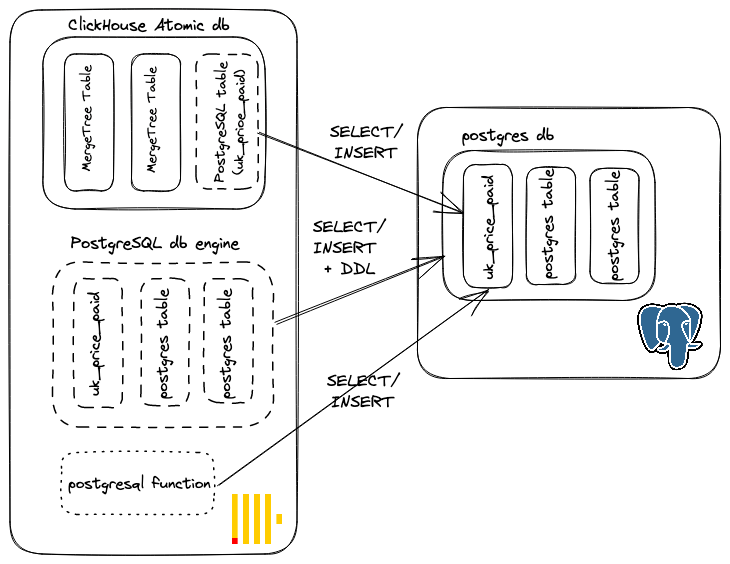
We have a few ways to access data in Postgres with ClickHouse:
- Utilise the postgresql function. This creates a connection per query and streams into ClickHouse. Simple WHERE clauses are pushed down where possible (e.g. utilising a ClickHouse-specific function prevents pushdown) to identify the matching rows. Once the matching rows are returned, aggregations, JOINs, sorting, and LIMIT clauses are performed in ClickHouse.
- Create a table in ClickHouse using the PostgreSQL table engine. This allows an entire Postgres table to be mirrored in ClickHouse. Implementation-wise, this is no different from the postgresql function, i.e., the selection of rows is pushed down where possible, but it simplifies query syntax considerably - we can use the table like any other within ClickHouse.
- Create a database using the PostgreSQL database engine. In this case, we mirror the entire database and can utilize all of its respective tables. This also allows us to execute DDL commands to modify and drop columns in tables in the underlying PostgreSQL instance.
The first two of these are available in ClickHouse Cloud, with the latter due to be exposed soon. Let's demonstrate the above previous functions, re-running the queries from ClickHouse. Here the data remains in PostgreSQL, with the data streamed into ClickHouse for the period of the query execution only - it is not persisted in a local MergeTree table. This is predominantly useful for ad-hoc analysis and for joining small datasets to local tables. Note that our ClickHouse Cloud instance is in the same AWS region as our Supabase database, to minimize network latency and maximize bandwidth connectivity.
Average price per year for flats in the UK
SELECT
	toYear(date) AS year,
	round(avg(price)) AS price
FROM postgresql('db.zcxfcrchxescrtxsnxuc.supabase.co', 'postgres', 'uk_price_paid', 'postgres', '')
WHERE type = 'flat'
GROUP BY year
ORDER BY year ASC


┌─year─┬──price─┐
│ 1995 │  59004 │
│ 1996 │  63913 │
...
│ 2021 │ 310626 │
│ 2022 │ 298977 │
└──────┴────────┘

28 rows in set. Elapsed: 26.408 sec. Processed 4.98 million rows, 109.59 MB (175.34 thousand rows/s., 3.86 MB/s.)
The above query again results in a full scan in Postgres, with the results streamed to ClickHouse where they are aggregated. This delivers comparable performance to the query being executed directly on Postgres.
Most expensive postcodes in a city
SELECT
      postcode1,
      round(avg(price)) AS price
FROM postgresql('db.zcxfcrchxescrtxsnxuc.supabase.co', 'postgres', 'uk_price_paid', 'postgres', '') WHERE town='BRISTOL' AND postcode1 != ''
GROUP BY postcode1
ORDER BY price DESC LIMIT 10

┌─postcode1─┬──price─┐
│ BS1   	│ 410726 │
│ BS19  	│ 369000 │
│ BS18  	│ 337000 │
│ BS40  	│ 323854 │
│ BS9   	│ 313248 │
│ BS8   	│ 301595 │
│ BS41  	│ 300802 │
│ BS6   	│ 272332 │
│ BS35  	│ 260563 │
│ BS36  	│ 252943 │
└───────────┴────────┘

10 rows in set. Elapsed: 2.362 sec. Processed 424.39 thousand rows, 15.11 MB (143.26 thousand rows/s., 5.10 MB/s.)
This time the town clause is pushed down to Postgres where the index is exploited, reducing the amount of data to return to ClickHouse. The performance is largely determined by the bandwidth and connectivity of the two databases. We experience some overhead, despite the same AWS region, but the performance remains comparable.
Postcodes in London with the largest percentage price change in the last 20 yrs
SELECT
	med_2002.postcode1,
	median_2002,
	median_2022,
	round(((median_2022 - median_2002) / median_2002) * 100) AS percent_change
FROM
(
	SELECT
    	postcode1,
    	median(price) AS median_2002
	FROM postgresql('db.zcxfcrchxescrtxsnxuc.supabase.co', 'postgres', 'uk_price_paid', 'postgres', '')
	WHERE (town = 'LONDON') AND (toYear(date) = '2002')
	GROUP BY postcode1
) AS med_2002
INNER JOIN
(
	SELECT
    	postcode1,
    	median(price) AS median_2022
	FROM postgresql('db.zcxfcrchxescrtxsnxuc.supabase.co', 'postgres', 'uk_price_paid', 'postgres', '')
	WHERE (town = 'LONDON') AND (toYear(date) = '2022')
	GROUP BY postcode1
) AS med_2022 ON med_2002.postcode1 = med_2022.postcode1
ORDER BY percent_change DESC
LIMIT 10

┌─postcode1─┬─median_2002─┬─median_2022─┬─percent_change─┐
│ EC3A  	│  	260000 │	16000000 │       	6054 │
│ SW1A  	│  	525000 │	17500000 │       	3233 │
│ EC2M  	│  	250000 │   4168317.5 │       	1567 │
│ EC3R  	│  	230000 │ 	2840000 │       	1135 │
│ W1S   	│  	590000 │ 	6410000 │        	986 │
│ WC2A  	│  	255000 │ 	2560000 │        	904 │
│ W1K   	│  	550000 │ 	5000000 │        	809 │
│ W1F   	│  	280000 │ 	2032500 │        	626 │
│ WC1B  	│  	390000 │ 	2205000 │        	465 │
│ W1J   	│  	497475 │ 	2800000 │        	463 │
└───────────┴─────────────┴─────────────┴────────────────┘

10 rows in set. Elapsed: 59.859 sec. Processed 4.25 million rows, 157.75 MB (71.04 thousand rows/s., 2.64 MB/s.)
This query is appreciably slower than the direct Postgres execution. This can be largely attributed to the fact the toYear(date) is not pushed down to Postgres, where the (extract(year from date)) index can be exploited. This query also streams the results from Postgres twice - once for each side of the join.
We can, however, rewrite this query to use ClickHouse’s conditional aggregate function medianIf. As well as being simpler and more intuitive, it is also faster by avoiding the join and double reading of the Postgres table.
SELECT
	postcode1,
	medianIf(price, toYear(date) = 2002) AS median_2002,
	medianIf(price, toYear(date) = 2022) AS median_2022,
	round(((median_2022 - median_2002) / median_2002) * 100) AS percent_change
FROM postgresql('db.zcxfcrchxescrtxsnxuc.supabase.co', 'postgres', 'uk_price_paid', 'postgres', '')
WHERE town = 'LONDON'
GROUP BY postcode1
ORDER BY percent_change DESC
LIMIT 10

┌─postcode1─┬─median_2002─┬─median_2022─┬─percent_change─┐
│ EC3A  	│  	260000 │	16000000 │       	6054 │
│ SW1A  	│  	525000 │	17500000 │       	3233 │
│ EC2M  	│  	250000 │   4168317.5 │       	1567 │
│ EC3R  	│  	230000 │ 	2840000 │       	1135 │
│ W1S   	│  	590000 │ 	6410000 │        	986 │
│ WC2A  	│  	255000 │ 	2560000 │        	904 │
│ W1K   	│  	550000 │ 	5000000 │        	809 │
│ W1F   	│  	280000 │ 	2032500 │        	626 │
│ WC1B  	│  	390000 │ 	2205000 │        	465 │
│ W1J   	│  	497475 │ 	2800000 │        	463 │
└───────────┴─────────────┴─────────────┴────────────────┘

10 rows in set. Elapsed: 36.166 sec. Processed 2.13 million rows, 78.88 MB (58.79 thousand rows/s., 2.18 MB/s.)
Utilizing a table engine simplifies this syntactically. The simplest means of creating this is using the CREATE AS syntax below. When ClickHouse creates the table locally, types in Postgres will be mapped to equivalent ClickHouse types - as shown by the subsequent SHOW CREATE AS statement. Note we use the setting external_table_functions_use_nulls = 0, to ensure Null values are represented as their default values (instead of Null). If set to 1 (the default), ClickHouse will create Nullable variants of each column.
CREATE TABLE uk_price_paid_postgresql AS postgresql('db.zcxfcrchxescrtxsnxuc.supabase.co', 'postgres', 'uk_price_paid', 'postgres', '')

SHOW CREATE TABLE uk_price_paid_postgresql

CREATE TABLE default.uk_price_paid_postgresql
(
	`id` Int32,
	`price` Int32,
	`date` Date,
	`postcode1` String,
	`postcode2` String,
	`type` String,
	`is_new` Int16,
	`duration` String,
	`addr1` String,
	`addr2` String,
	`street` String,
	`locality` String,
	`town` String,
	`district` String,
	`county` String
) AS postgresql('db.zcxfcrchxescrtxsnxuc.supabase.co', 'postgres', 'uk_price_paid', 'postgres', '[HIDDEN]')
This makes our earlier query a little simpler, with the same results.
SELECT
	postcode1,
	medianIf(price, toYear(date) = 2002) AS median_2002,
	medianIf(price, toYear(date) = 2022) AS median_2022,
	round(((median_2022 - median_2002) / median_2002) * 100) AS percent_change
FROM uk_price_paid_postgresql
WHERE town = 'LONDON'
GROUP BY postcode1
ORDER BY percent_change DESC
LIMIT 10

┌─postcode1─┬─median_2002─┬─median_2022─┬─percent_change─┐
│ EC3A  	│  	260000 │	16000000 │       	6054 │
│ SW1A  	│  	525000 │	17500000 │       	3233 │
│ EC2M  	│  	250000 │   4168317.5 │       	1567 │
│ EC3R  	│  	230000 │ 	2840000 │       	1135 │
│ W1S   	│  	590000 │ 	6410000 │        	986 │
│ WC2A  	│  	255000 │ 	2560000 │        	904 │
│ W1K   	│  	550000 │ 	5000000 │        	809 │
│ W1F   	│  	280000 │ 	2032500 │        	626 │
│ WC1B  	│  	390000 │ 	2205000 │        	465 │
│ W1J   	│  	497475 │ 	2800000 │        	463 │
└───────────┴─────────────┴─────────────┴────────────────┘

10 rows in set. Elapsed: 28.531 sec. Processed 2.13 million rows, 78.88 MB (74.52 thousand rows/s., 2.76 MB/s.)
We could define our table types explicitly and avoid using the SHOW CREATE AS.
CREATE TABLE default.uk_price_paid_v2
(
	`price` UInt32,
	`date` Date,
	`postcode1` String,
	`postcode2` String,
	`type` Enum8('other' = 0, 'terraced' = 1, 'semi-detached' = 2, 'detached' = 3, 'flat' = 4),
	`is_new` UInt8,
	`duration` Enum8('unknown' = 0, 'freehold' = 1, 'leasehold' = 2),
	`addr1` String,
	`addr2` String,
	`street` String,
	`locality` String,
	`town` String,
	`district` String,
	`county` String
)
ENGINE = PostgreSQL('db.zcxfcrchxescrtxsnxuc.supabase.co', 'postgres', 'uk_price_paid', 'postgres', '')
There are a few takeaways concerning performance:
- ClickHouse can push down filter clauses if they are simple i.e. =, !=, >, >=, <, <=, and IN, allowing indexes in Postgres to be potentially exploited. If they involve ClickHouse-specific functions (or if Postgres determines a full scan is the best execution method), a full table scan will be performed, and Postgres indexes will not be exploited. This can lead to large differences in performance depending on where the query is run due to the need to stream the entire dataset to ClickHouse. If bandwidth connectivity is not an issue, and Postgres would need to perform a full scan even if the query was executed directly, then differences in performance will be less appreciable.
- If using the
postgresfunction or table engine, be cognizant of the number of queries required from Postgres. In our earlier example, we minimized the use of the function to speed up queries. Balance this against being able to exploit Postgres indexes to minimize the data streamed to ClickHouse.
Postgres to ClickHouse
Up to now, we’ve only pushed queries down to Postgres. While occasionally useful for ad-hoc analysis and querying small datasets, you will eventually want to exploit ClickHouse’s MergeTree table and its associated performance on analytical queries. Moving data between Postgres and ClickHouse is as simple as using the INSERT INTO x SELECT FROM syntax.
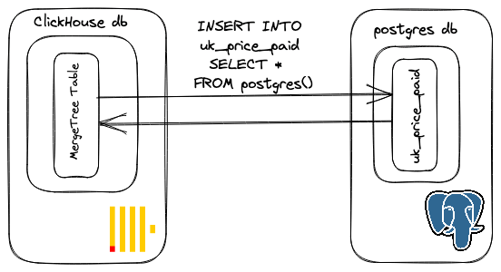
In the example below, we create a table and attempt to insert the data from our Supabase-hosted Postgres instance:
CREATE TABLE default.uk_price_paid
(
   `price` UInt32,
   `date` Date,
   `postcode1` LowCardinality(String),
   `postcode2` LowCardinality(String),
   `type` Enum8('other' = 0, 'terraced' = 1, 'semi-detached' = 2, 'detached' = 3, 'flat' = 4),
   `is_new` UInt8,
   `duration` Enum8('unknown' = 0, 'freehold' = 1, 'leasehold' = 2),
   `addr1` String,
   `addr2` String,
   `street` LowCardinality(String),
   `locality` LowCardinality(String),
   `town` LowCardinality(String),
   `district` LowCardinality(String),
   `county` LowCardinality(String)
)
ENGINE = MergeTree
ORDER BY (type, town, postcode1, postcode2)

INSERT INTO uk_price_paid_v2 SELECT * EXCEPT id
FROM postgresql('db.zcxfcrchxescrtxsnxuc.supabase.co', 'postgres', 'uk_price_paid', 'postgres', '')

↘ Progress: 21.58 million rows, 3.99 GB (177.86 thousand rows/s., 32.89 MB/s.)                                                                                                                                                                                                                   	(0.5 CPU, 39.00 MB RAM)
0 rows in set. Elapsed: 121.361 sec. Processed 21.58 million rows, 3.99 GB (177.86 thousand rows/s., 32.89 MB/s.)

Received exception from server (version 22.11.1):
Code: 1001. DB::Exception: Received from oxvdst5xzq.us-west-2.aws.clickhouse.cloud:9440. DB::Exception: pqxx::sql_error: Failure during '[END COPY]': ERROR:  canceling statement due to statement timeout
. (STD_EXCEPTION)
In our example above, we attempted to pull all 28m rows from Supabase. Unfortunately, due to Supabase imposing a global time limit on queries of 2 minutes this query doesn’t complete. To work around this, we filter on the type column to obtain subsets of the data - each of these queries can exploit the filter pushed down and complete in under 2 minutes.
INSERT INTO uk_price_paid SELECT * EXCEPT id FROM postgresql('db.zcxfcrchxescrtxsnxuc.supabase.co', 'postgres', 'uk_price_paid', 'postgres', '') WHERE type = 'other'

INSERT INTO uk_price_paid SELECT * EXCEPT id FROM postgresql('db.zcxfcrchxescrtxsnxuc.supabase.co', 'postgres', 'uk_price_paid', 'postgres', '') WHERE type = 'detached'

INSERT INTO uk_price_paid SELECT * EXCEPT id FROM postgresql('db.zcxfcrchxescrtxsnxuc.supabase.co', 'postgres', 'uk_price_paid', 'postgres', '') WHERE type = 'flat'

INSERT INTO uk_price_paid SELECT * EXCEPT id FROM postgresql('db.zcxfcrchxescrtxsnxuc.supabase.co', 'postgres', 'uk_price_paid', 'postgres', '') WHERE type = 'terraced'

INSERT INTO uk_price_paid SELECT * EXCEPT id FROM postgresql('db.zcxfcrchxescrtxsnxuc.supabase.co', 'postgres', 'uk_price_paid', 'postgres', '') WHERE type = 'semi-detached'
As of the type of writing, overcoming these query limits requires the user to split their data on a column of appropriate cardinality. However, other services, or self-managed instances, may not impose this restriction.
Using our new MergeTree table, we can execute our earlier queries directly in ClickHouse.
The average price per year for flats in the UK
SELECT toYear(date) AS year, round(avg(price)) AS price FROM uk_price_paid WHERE type = 'flat' GROUP BY year ORDER BY year ASC ┌─year─┬──price─┐ │ 1995 │ 59004 │ │ 1996 │ 63913 │ │ 1997 │ 72302 │ │ 1998 │ 80775 │ │ 1999 │ 93646 │ ... │ 2019 │ 300938 │ │ 2020 │ 319547 │ │ 2021 │ 310626 │ │ 2022 │ 298977 │ └──────┴────────┘ 28 rows in set. Elapsed: 0.079 sec. Processed 5.01 million rows, 35.07 MB (63.05 million rows/s., 441.37 MB/s.)✎
Most expensive postcodes in a city
SELECT postcode1, round(avg(price)) AS price FROM uk_price_paid WHERE (town = 'BRISTOL') AND (postcode1 != '') GROUP BY postcode1 ORDER BY price DESC LIMIT 10 ┌─postcode1─┬──price─┐ │ BS1 │ 410726 │ │ BS19 │ 369000 │ │ BS18 │ 337000 │ │ BS40 │ 323854 │ │ BS9 │ 313248 │ │ BS8 │ 301595 │ │ BS41 │ 300802 │ │ BS6 │ 272332 │ │ BS35 │ 260563 │ │ BS36 │ 252943 │ └───────────┴────────┘ 10 rows in set. Elapsed: 0.077 sec. Processed 27.69 million rows, 30.21 MB (358.86 million rows/s., 391.49 MB/s.)✎
Postcodes in London with the largest percentage price change in the last 20 yrs
SELECT postcode1, medianIf(price, toYear(date) = 2002) AS median_2002, medianIf(price, toYear(date) = 2022) AS median_2022, round(((median_2022 - median_2002) / median_2002) * 100) AS percent_change FROM uk_price_paid WHERE town = 'LONDON' GROUP BY postcode1 ORDER BY percent_change DESC ┌─postcode1─┬─median_2002─┬─median_2022─┬─percent_change─┐ │ EC3A │ 260000 │ 16000000 │ 6054 │ │ SW1A │ 525000 │ 17500000 │ 3233 │ │ EC2M │ 250000 │ 4168317.5 │ 1567 │ │ EC3R │ 230000 │ 2840000 │ 1135 │ │ W1S │ 590000 │ 6410000 │ 986 │ 191 rows in set. Elapsed: 0.062 sec. Processed 2.62 million rows, 19.45 MB (41.98 million rows/s., 311.48 MB/s.)✎
The difference here in query performance is dramatic. In the interests of transparency, there are reasons for this beyond simply “ClickHouse is faster on analytical queries”:
- This is a developer instance in ClickHouse Cloud with 8GB of RAM and 2 cores. We don’t have visibility regarding the resources assigned to each Supabase instance, but this is likely more.
- All queries were executed 5x with the minimum of these used. This ensures that we use both databases' “hot” performance and exploit any file system caches.
- We have optimized our primary key for our ClickHouse table to minimize the number of rows scanned.
Despite these differences, ClickHouse clearly excels on linear scans and analytical-type queries, especially when the primary index can be exploited - this is reinforced by our more rigorous benchmarks.
Conclusion
In the first part of this blog series, we have shown how ClickHouse and Postgres are complementary, demonstrating with examples how data can be moved effortlessly between them using the native ClickHouse functions and table engine. In the next part, we will show how Postgres can be used to power dictionaries which are automatically kept in sync and used to accelerate join queries.
In the meantime, if you want to learn more about out Postgres integration we have free training course on data ingestion which covers these topics extensively.