Introduction
Generating test data can be challenging, given that real-world data is never random. While the generateRandom() function is useful as a fast means of populating a table, generating data with real-world properties will help test a system in a more realistic context. Real data has unique properties - a certain range limits it, it gravitates towards specific values, and is never evenly distributed over time. Since 22.10, powerful functions have been added to ClickHouse to generate random data with a high level of flexibility. Let’s take a look at some of these and generate some useful test data!
All examples in this post can be reproduced in our play.clickhouse.com environment. Alternatively, all of the examples in this post were created on a developer instance in ClickHouse Cloud where you can spin up a cluster on a free trial in minutes, let us deal with the infrastructure, and get querying!
Knowledge of probability distributions, whilst useful, is not essential to make use of the content in this blog post. Most examples can be reused with a simple copy and paste. We will first introduce the random functions, each with a simple example, before using them in a combined example to generate a practically useful dataset.
Uniform random distributions
In some cases, data can be uniformly distributed, i.e., the interval between data points is constant. These functions have existed in ClickHouse for some time but remain useful for columns with predictable distributions.
Canonical random in 0…1 range
Clickhouse has a canonical random function that all databases and programming languages have. This function returns pseudo-random values from 0 (inclusive) to 1 (not exclusive) that are uniformly distributed:
SELECT randCanonical()✎
Random numbers in X…Y range
To generate random numbers within a given range (including lower number, excluding upper value), we can use randUniform:
This function generates a random float number in the `5...9.9(9)` range. The `randUniform()` function uses a uniform distribution, meaning we will see the same amount of random values across all the given range (when we call the function many times). In other words - this gives us truly random numbers within a given range.SELECT randUniform(5,10)✎
Random integers
To generate random integer numbers, we can round with a floor() function:
SELECT floor(randUniform(5, 10)) AS r✎
This outputs random numbers in the 5...9 range.
Note: Due to the nature of a uniform distribution, we can't use
round()here because we'll end up getting numbers from 6 to 9 (everything that's within a given range) more frequently than 5 and 10 (range edges).
Non-uniform random distributions
The 22.10 release of ClickHouse delivers random functions capable of generating non-uniform (and continuous) distributions. Non-uniform distribution means that by calling such a function many times, we get some random numbers more frequently than others. The nature of the generated distribution is function specific. Read more on non-uniform distributions and their common applications.
The most popular distribution is normal, which is implemented by randNormal() function:
SELECT randNormal(100, 5)✎
This function takes a mean value as the first argument and variance as the second, outputting float numbers around a mean - 100 in our example above. Let’s take a look at how these generated numbers are distributed:
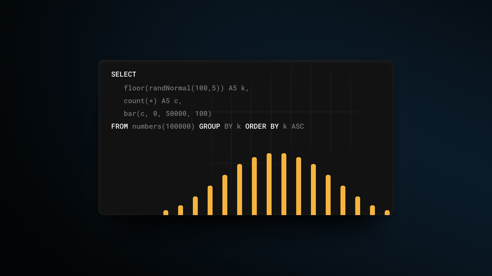
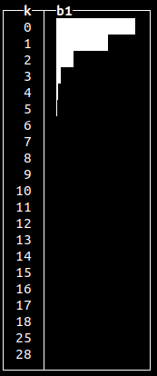
SELECT floor(randNormal(100, 5)) AS k, count(*) AS c, bar(c, 0, 50000, 100) FROM numbers(100000) GROUP BY k ORDER BY k ASC 45 rows in set. Elapsed: 0.005 sec. Processed 130.82 thousand rows, 1.05 MB (24.44 million rows/s., 195.53 MB/s.)✎
Here, we generate 100k random numbers using randNormal(), round them and count how many times each number occurs. We see that most of the time, the function will generate a random number closer to the given mean (which is precisely how normal distribution works).
Normal distributions occur when we sum many independent variables, e.g., aggregate types of errors in our system. Other non-uniform random distributions available are:
Generating random data
We can use any of the given random generators according to our requirements and populate our tables with test data. Let’s populate a purchases table representing product sales:
CREATE TABLE purchases
(
    `dt` DateTime,
    `customer_id` UInt32,
    `total_spent` Float32
)
ENGINE = MergeTree
ORDER BY dt
We’ll use randExponential() function to generated data for the column total_spent to emulate the distribution of customer sales:
INSERT INTO purchases SELECT
    now() - randUniform(1, 1000000.),
    number,
    15 + round(randExponential(1 / 10), 2)
FROM numbers(1000000)
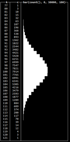
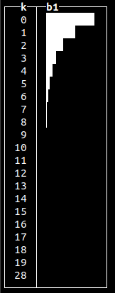
We’ve used serial numbers for customer IDs and uniform random shifts in time to spread the data. We can see the total_spent value is distributed accordingly to exponential law, gravitating to the value of 15 (assuming $15.00 is the lowest value that can be spent):
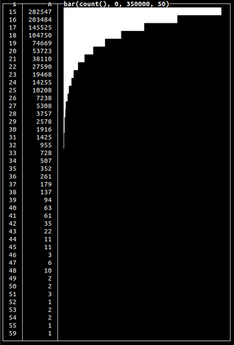
Note how we used the exponential distribution to get a gradual decrease in total spend. We could use the normal distribution (using randNormal() function) or any other to get a different peak and form.
Generating time-distributed data
While in our previous examples, we used the random distribution to model values, we can also model time. Let’s say we collect client events into the following table:
CREATE TABLE events
(
    `dt` DateTime,
    `event` String
)
ENGINE = MergeTree
ORDER BY dt
In reality, more events might occur at specific hours of the day. The Poisson distribution is a good way to model a series of independent events in time. To simulate a distribution of time, we just have to add generated random values to the time column:
INSERT INTO events SELECT
    toDateTime('2022-12-12 12:00:00') - (((12 + randPoisson(12)) * 60) * 60),
    'click'
FROM numbers(100000)

0 rows in set. Elapsed: 0.014 sec. Processed 100.00 thousand rows, 800.00 KB (7.29 million rows/s., 58.34 MB/s.)
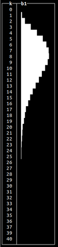
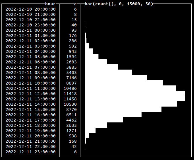
Here, we’re inserting 100k click events that are distributed over approximately a 24-hour period, with midday being the time when there is a peak of events (12:00 in our example):
SELECT toStartOfHour(dt) AS hour, count(*) AS c, bar(c, 0, 15000, 50) FROM blogs.events GROUP BY hour ORDER BY hour ASC 750 rows in set. Elapsed: 0.095 sec. Processed 20.10 million rows, 80.40 MB (211.36 million rows/s., 845.44 MB/s.)✎
In this case, instead of generating values, we used a random function to insert new records at a calculated point in time:
Generating time-dependent values
Building on the previous example, we can use a distribution to generate values that depend on time. For example, suppose we want to emulate hardware metrics collection, like CPU utilization or RAM usage, into the following table:
CREATE TABLE metrics
(
    `name` String,
    `dt` DateTime,
    `val` Float32
)
ENGINE = MergeTree
ORDER BY (name, dt)
In real-world cases, we’ll certainly have peak hours when our CPU is fully loaded and periods of lower load. To model this, we can calculate both metric values and a time point value using a random function of the required distribution:
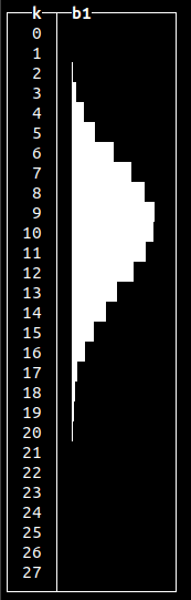
INSERT INTO metrics SELECT
    'cpu',
    t + ((60 * 60) * randCanonical()) AS t,
    round(v * (0.95 + (randCanonical() / 20)), 2) AS v
FROM
(
    SELECT
        toDateTime('2022-12-12 12:00:00') - INTERVAL k HOUR
 AS t,
        round((100 * c) / m, 2) AS v
    FROM
    (
        SELECT
            k,
            c,
            max(c) OVER () AS m
        FROM
        (
            SELECT
                floor(randBinomial(24, 0.5) - 12) AS k,
                count(*) AS c
            FROM numbers(1000)
            GROUP BY k
            ORDER BY k ASC
        )
    )
) AS a
INNER JOIN numbers(1000000) AS b ON 1 = 1

0 rows in set. Elapsed: 3.952 sec. Processed 1.05 million rows, 8.38 MB (265.09 thousand rows/s., 2.12 MB/s.)
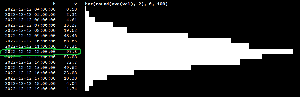
Here, we generate 1k binomially distributed random values to get each generated number and its associated count. We then compute the max of these values using a window max function, adding this as a column to each result. Finally, in the outer query, we’re generating a metric value based on that count divided by the max to get a random value in the range of 0...100, corresponding to possible CPU load data. We also add noise to time, and val using randCanonical() and join on numbers to generate 1m metric events. Let’s check how our values are distributed:
SELECT toStartOfHour(dt) AS h, round(avg(val), 2) AS v, bar(v, 0, 100) FROM metrics GROUP BY h ORDER BY h ASC✎
Generating multi-modal distributions
All of our previous examples produced data with a single peak or optima. Multi-modal distributions contain multiple peaks and are useful for simulating real-world events such as multiple seasonal peaks of sales. We can achieve this by grouping generated values by a certain serial number to repeat our generated data:
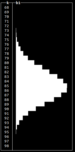
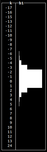
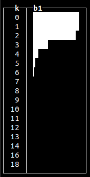
SELECT floor(randBinomial(24, 0.75)) AS k, count(*) AS c, number % 3 AS ord, bar(c, 0, 10000) FROM numbers(100000) GROUP BY k, ord ORDER BY ord ASC, k ASC✎
This will repeat our binomially distributed data three times:
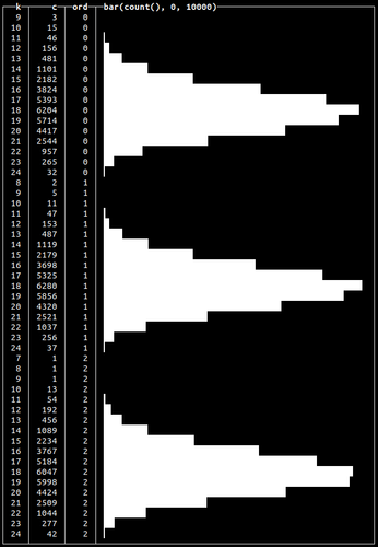
This is an aggregated query example. We’ll use this approach again later to actually insert multi-model distributed data into a table in the “Generating Click Stream test data” section.
Simulating binary states
The randBernoulli() function returns 0 or 1 based on a given probability e.g. if we want to get 1 90% of the time, we use:
SELECT randBernoulli(0.9)✎
This can be useful when generating data for binary states such as failed or successful transactions:
SELECT If(randBernoulli(0.95), 'success', 'failure') AS status, count(*) AS c FROM numbers(1000) GROUP BY status ┌─status──┬───c─┐ │ failure │ 49 │ │ success │ 951 │ └─────────┴─────┘ 2 rows in set. Elapsed: 0.004 sec. Processed 1.00 thousand rows, 8.00 KB (231.05 thousand rows/s., 1.85 MB/s.)✎
Here we generate 95% of success states and only 5% of failure.
Generating random values for Enums
We can use a combination of an array and random function to get values from a certain subset and use this to populate an ENUM column:
SELECT ['200', '404', '502', '403'][toInt32(randBinomial(4, 0.1)) + 1] AS http_code, count(*) AS c FROM numbers(1000) GROUP BY http_code ┌─http_code─┬───c─┐ │ 403 │ 5 │ │ 502 │ 43 │ │ 200 │ 644 │ │ 404 │ 308 │ └───────────┴─────┘ 4 rows in set. Elapsed: 0.004 sec. Processed 1.00 thousand rows, 8.00 KB (224.14 thousand rows/s., 1.79 MB/s.)✎
Here we used the binomial distribution to get the number of requests with one of 4 possible HTTP response codes. We would typically expect more 200s than errors and hence model as such.
Generating random strings
Clickhouse also allows generating random strings using randomString(), randomStringUTF8() and randomPrintableASCII() functions. All of the functions accept string length as an argument. To create a dataset with random strings, we can combine string generation with random functions to get strings of arbitrary length. Below we use this approach to generate 10 random strings, of readable characters, of 5 to 25 symbols in length:
SELECT randomPrintableASCII(randUniform(5, 25)) AS s, length(s) AS length FROM numbers(10) ┌─s────────────────────┬─length─┐ │ (+x3e#Xc>VB~kTAtR|! │ 19 │ │ "ZRKa_ │ 6 │ │ /$q4I/^_-)m;tSQ&yGq5 │ 20 │ │ 2^5$2}6(H>dr │ 12 │ │ Gt.GO │ 5 │ │ 0WR4_6V1"N^/."DtB! │ 18 │ │ ^0[!uE │ 6 │ │ A&Ks|MZ+P^P^rd\ │ 15 │ │ '-K}|@y$jw0z?@?m?S │ 18 │ │ eF(^"O&'^' │ 10 │ └──────────────────────┴────────┘ 10 rows in set. Elapsed: 0.001 sec.✎
Generating noisy data
In the real world, data will always contain errors. This can be simulated in Clickhouse using the fuzzBits() function. This function can generate erroneous data based on user-specified valid values by randomly shifting bits with a specified probability. Let’s say we want to add errors to a string field values. The following will randomly generate errors based on our initial value:
SELECT fuzzBits('Good string', 0.01) FROM numbers(10) ┌─fuzzBits('Good string', 0.01)─┐ │ Good�string │ │ g/od string │ │ Goe string │ │ Good strhfg │ │ Good0string │ │ Good0spring │ │ Good string │ │ �ood string │ │ Good string │ │ Good string │ └───────────────────────────────┘ 10 rows in set. Elapsed: 0.001 sec.✎
Be sure to tune the probability since the number of generated errors depends on the length of values you pass to the function. Use lower values for a probability of getting fewer errors:
SELECT IF(fuzzBits('Good string', 0.001) = 'Good string', 1, 0) AS has_errors, count(*) FROM numbers(1000) GROUP BY has_errors ┌─has_errors─┬─count()─┐ │ 0 │ 295 │ │ 1 │ 705 │ └────────────┴─────────┘ 2 rows in set. Elapsed: 0.004 sec. Processed 1.00 thousand rows, 8.00 KB (276.99 thousand rows/s., 2.22 MB/s.)✎
Here, we’ve used 0.001 probability to get ~25% of values with errors:
Generating a real dataset
To wrap everything up, let’s simulate a click stream for 30 days that has a close-to-real-world distribution within a day with peaks at noon. We’ll use a normal distribution for this. Each event will also have one of two possible states: success or fail, distributed using the Bernoulli function. Our table:
CREATE TABLE click_events
(
    `dt` DateTime,
    `event` String,
    `status` Enum8('success' = 1, 'fail' = 2)
)
ENGINE = MergeTree
ORDER BY dt
Let’s populate this table with 10m events:
INSERT INTO click_events SELECT
    (parseDateTimeBestEffortOrNull('12:00') - toIntervalHour(randNormal(0, 3))) - toIntervalDay(number % 30),
    'Click',
    ['fail', 'success'][randBernoulli(0.9) + 1]
FROM numbers(10000000)

0 rows in set. Elapsed: 3.726 sec. Processed 10.01 million rows, 80.06 MB (2.69 million rows/s., 21.49 MB/s.)
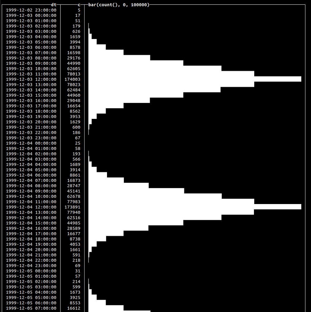
We’ve used randBernoulli() with a 90% success probability, so we’ll have success value for the status column 9 out of 10 times. We’ve used randNormal() to generate the distribution of the events. Let’s visualize that data with the following query:
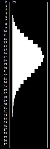
SELECT dt, count(*) AS c, bar(c, 0, 100000) FROM click_events GROUP BY dt ORDER BY dt ASC 722 rows in set. Elapsed: 0.045 sec. Processed 10.00 million rows, 40.00 MB (224.41 million rows/s., 897.64 MB/s.)✎
This will yield the following output:
Summary
Using powerful random functions available since 22.10, we have shown how to generate data of a realistic nature. This data can be used to help test your solutions on close-to-the-real-world data instead of irrelevant generated sets.