This was originally a post by ensemble analytics, who have kindly allowed republishing of this content. We welcome posts from our community and thank them for their contributions.
Introduction
When doing statistical analysis or data science work, the first inclination is usually to break into a programming language such as Python or R at the earliest opportunity.
When we use ClickHouse however, we prefer to take things as far as possible using just the database. By doing this, we can rely on the power of ClickHouse to crunch numbers quickly, and reduce or even totally avoid the amount of code that we need to write. This also means that we can work with smaller in memory datasets on the client side and avoid the need for distributed computation.
A good example of this is forecasting. ClickHouse implements two machine learning functions - Stochastic Linear Regression (stochasticLinearRegression) which can be used for fitting the model, and a function (evalMLMethod) which can be used for subsequent inference directly within the database.
Of course there are more sophisticated forecasting models and more flexibility once you break out of SQL into a fully-fledged programming language, but this technique certainly has it's uses and performs well in our demonstration scenario here.
Dataset
To demonstrate, we are going to use a simple flight departure dataset which contains a monthly time series of the number of passengers departing from different airports using various airlines.
Our aim will be to take this data and use it forecast the same data into the future.
We will aim to build a model using data from 2008 to 2015, and then test the performance of the model between 2015 and 2018. Finally, we will then forecast beyond the period through till 2021.
Our source data has the following structure:
SELECT *
FROM flight_data
LIMIT 10

┌─AIRLINE─┬─DEPARTURE_AIRPORT─┬──────MONTH─┬─PASSENGERS─┐
│ Delta   │ DIA               │ 2008-01-01 │        434 │
│ Delta   │ DIA               │ 2008-02-01 │        475 │
│ Delta   │ DIA               │ 2008-03-01 │        531 │
│ Delta   │ DIA               │ 2008-04-01 │        509 │
│ Delta   │ DIA               │ 2008-05-01 │        472 │
│ Delta   │ DIA               │ 2008-06-01 │        562 │
│ Delta   │ DIA               │ 2008-07-01 │        642 │
│ Delta   │ DIA               │ 2008-08-01 │        642 │
│ Delta   │ DIA               │ 2008-09-01 │        596 │
│ Delta   │ DIA               │ 2008-10-01 │        503 │
└─────────┴───────────────────┴────────────┴────────────┘

10 rows in set. Elapsed: 0.002 sec. Processed 4.62 thousand rows, 151.54 KB (2.16 million rows/s., 70.86 MB/s.)
Peak memory usage: 229.15 KiB.
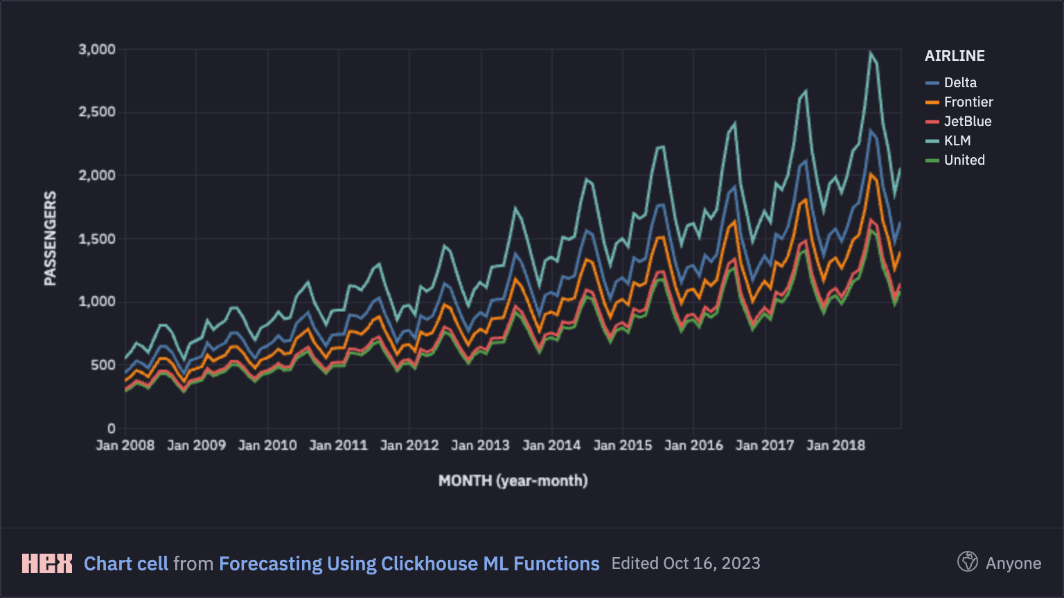
When plotted, the data looks like this, showing how all airlines are carrying an increased number of passengers over time together with a significant seasonality effect.
Data Preparation
Our forecasting model uses 13 deterministic features: a linear time trend and 12 dummy (or one-hot encoded) variables representing the 12 months of the year. We exclude the constant term (or intercept) in order to avoid the "dummy variable trap".
The model predicts the logarithm of the number of passengers. The logarithmic transformation allows us to better capture the time-varying amplitude of the seasonal fluctuations.
CREATE VIEW
    data
AS WITH
    (select toDate(min(MONTH)) from flight_data) as start_date,
    (select toDate(max(MONTH)) from flight_data) as end_date
SELECT
    AIRLINE,
    DEPARTURE_AIRPORT,
    MONTH,
    toFloat64(log(PASSENGERS)) as Target,
    assumeNotNull(dateDiff('month', start_date, MONTH) / dateDiff('month', start_date, end_date)) as Trend,
    if(toMonth(toDate(MONTH)) = 1, 1, 0) as Dummy1,
    if(toMonth(toDate(MONTH)) = 2, 1, 0) as Dummy2,
    if(toMonth(toDate(MONTH)) = 3, 1, 0) as Dummy3,
    if(toMonth(toDate(MONTH)) = 4, 1, 0) as Dummy4,
    if(toMonth(toDate(MONTH)) = 5, 1, 0) as Dummy5,
    if(toMonth(toDate(MONTH)) = 6, 1, 0) as Dummy6,
    if(toMonth(toDate(MONTH)) = 7, 1, 0) as Dummy7,
    if(toMonth(toDate(MONTH)) = 8, 1, 0) as Dummy8,
    if(toMonth(toDate(MONTH)) = 9, 1, 0) as Dummy9,
    if(toMonth(toDate(MONTH)) = 10, 1, 0) as Dummy10,
    if(toMonth(toDate(MONTH)) = 11, 1, 0) as Dummy11,
    if(toMonth(toDate(MONTH)) = 12, 1, 0) as Dummy12
FROM
    flight_data
ORDER BY AIRLINE, DEPARTURE_AIRPORT, MONTH
This creates the following view which summarises our dependent and independent variables:
SELECT *
FROM data
LIMIT 10

┌─AIRLINE─┬─DEPARTURE_AIRPORT─┬──────MONTH─┬─────────────Target─┬────────────────Trend─┬─Dummy1─┬─Dummy2─┬─Dummy3─┬─Dummy4─┬─Dummy5─┬─Dummy6─┬─Dummy7─┬─Dummy8─┬─Dummy9─┬─Dummy10─┬─Dummy11─┬─Dummy12─┐
│ Delta   │ DIA               │ 2008-01-01 │ 6.0730445333335865 │                    0 │      1 │      0 │      0 │      0 │      0 │      0 │      0 │      0 │      0 │       0 │       0 │       0 │
│ Delta   │ DIA               │ 2008-02-01 │  6.163314804336003 │ 0.007633587786259542 │      0 │      1 │      0 │      0 │      0 │      0 │      0 │      0 │      0 │       0 │       0 │       0 │
│ Delta   │ DIA               │ 2008-03-01 │  6.274762021388925 │ 0.015267175572519083 │      0 │      0 │      1 │      0 │      0 │      0 │      0 │      0 │      0 │       0 │       0 │       0 │
│ Delta   │ DIA               │ 2008-04-01 │  6.232448016554782 │ 0.022900763358778626 │      0 │      0 │      0 │      1 │      0 │      0 │      0 │      0 │      0 │       0 │       0 │       0 │
│ Delta   │ DIA               │ 2008-05-01 │  6.156978985873825 │ 0.030534351145038167 │      0 │      0 │      0 │      0 │      1 │      0 │      0 │      0 │      0 │       0 │       0 │       0 │
│ Delta   │ DIA               │ 2008-06-01 │ 6.3315018500618665 │  0.03816793893129771 │      0 │      0 │      0 │      0 │      0 │      1 │      0 │      0 │      0 │       0 │       0 │       0 │
│ Delta   │ DIA               │ 2008-07-01 │  6.464588304624293 │  0.04580152671755725 │      0 │      0 │      0 │      0 │      0 │      0 │      1 │      0 │      0 │       0 │       0 │       0 │
│ Delta   │ DIA               │ 2008-08-01 │  6.464588304624293 │  0.05343511450381679 │      0 │      0 │      0 │      0 │      0 │      0 │      0 │      1 │      0 │       0 │       0 │       0 │
│ Delta   │ DIA               │ 2008-09-01 │  6.390240666362644 │ 0.061068702290076333 │      0 │      0 │      0 │      0 │      0 │      0 │      0 │      0 │      1 │       0 │       0 │       0 │
│ Delta   │ DIA               │ 2008-10-01 │  6.220590170138575 │  0.06870229007633588 │      0 │      0 │      0 │      0 │      0 │      0 │      0 │      0 │      0 │       1 │       0 │       0 │
└─────────┴───────────────────┴────────────┴────────────────────┴──────────────────────┴────────┴────────┴────────┴────────┴────────┴────────┴────────┴────────┴────────┴─────────┴─────────┴─────────┘

10 rows in set. Elapsed: 0.010 sec. Processed 13.86 thousand rows, 170.02 KB (1.37 million rows/s., 16.81 MB/s.)
Peak memory usage: 420.28 KiB.
Model Training
We use ClickHouse's stochasticLinearRegression algorithm, which trains a linear regression using gradient descent. We build 35 different models at the same time, one for each airline-airport combination.
CREATE VIEW model as SELECT
    AIRLINE,
    DEPARTURE_AIRPORT,
    stochasticLinearRegressionState(0.5, 0.01, 4, 'SGD')(
        Target, Trend, Dummy1, Dummy2, Dummy3, Dummy4, Dummy5, Dummy6, Dummy7, Dummy8, Dummy9, Dummy10, Dummy11, Dummy12
    ) as state
FROM train_data
GROUP BY AIRLINE, DEPARTURE_AIRPORT
As there is a small amount of data, the model is simply defined as a view. For bigger datasets, we may choose to materialize this as a table or a view.
Model Evaluation
We can now use the trained model to generate the forecasts over the test set and compare them to the actual values. At this stage we can also transform the data and the forecasts back to the original scale by taking the exponential.
SELECT
    a.MONTH as MONTH,
    a.AIRLINE as AIRLINE,
    a.DEPARTURE_AIRPORT as DEPARTURE_AIRPORT,
    toInt32(exp(a.Target)) as ACTUAL,
    toInt32(exp(evalMLMethod(b.state, Trend, Dummy1, Dummy2, Dummy3, Dummy4, Dummy5, Dummy6, Dummy7,
    Dummy8, Dummy9, Dummy10, Dummy11, Dummy12))) as FORECAST
FROM test_data as a
LEFT JOIN model as b
on a.AIRLINE = b.AIRLINE and a.DEPARTURE_AIRPORT = b.DEPARTURE_AIRPORT
If we compare the forecast and the actuals, we can see that the forecast performed well:
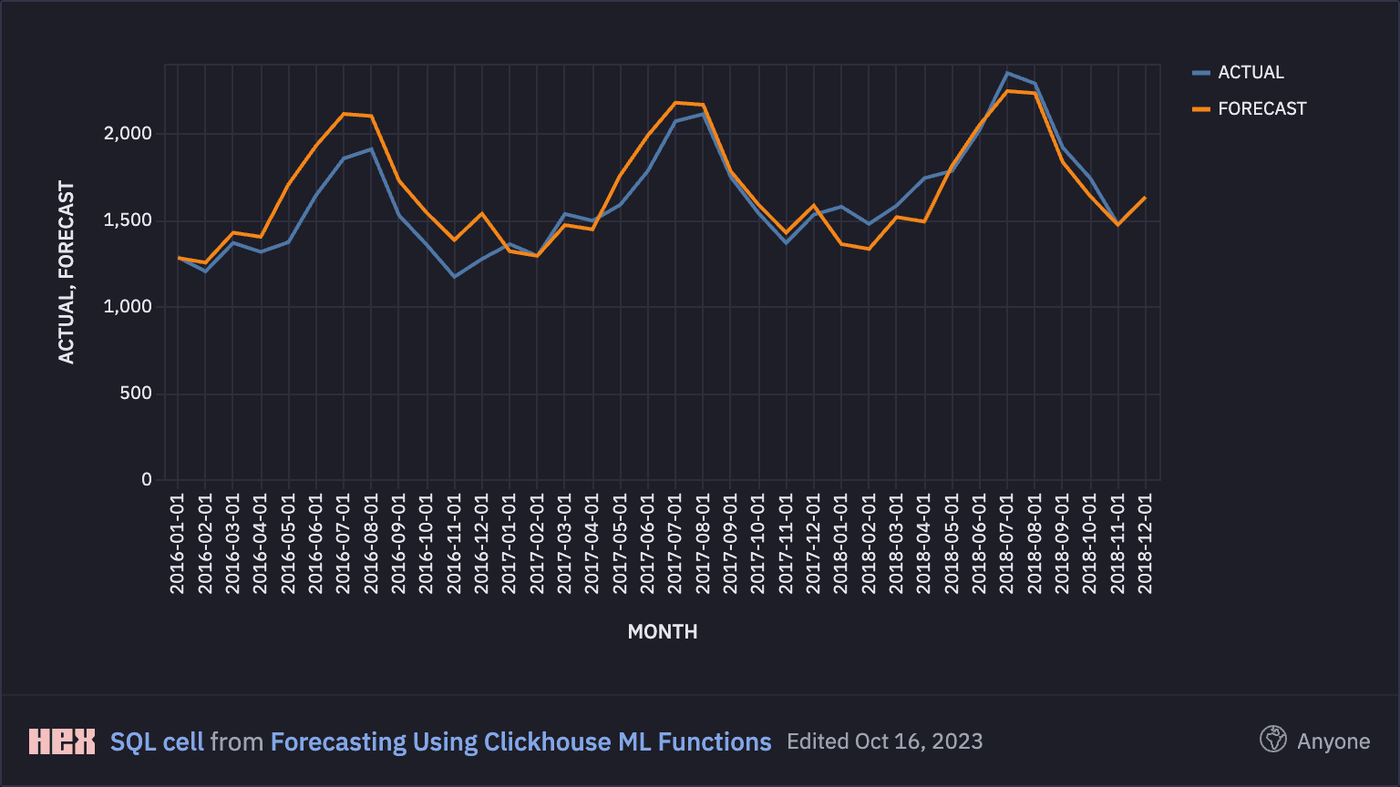
We can validate this by calculating the Mean Absolute Error (MAE) and Root Mean Squared Error (RMSE) of the forecasts for each airline-airport combination.
SELECT
    AIRLINE,
    DEPARTURE_AIRPORT,
    avg(abs(ERROR)) AS MAE,
    sqrt(avg(pow(ERROR, 2))) AS RMSE
FROM
(
    SELECT
        a.AIRLINE AS AIRLINE,
        a.DEPARTURE_AIRPORT AS DEPARTURE_AIRPORT,
        toInt32(exp(a.Target)) - toInt32(exp(evalMLMethod(b.state, Trend, Dummy1, Dummy2, Dummy3, Dummy4,
        Dummy5, Dummy6, Dummy7, Dummy8, Dummy9, Dummy10, Dummy11, Dummy12))) AS ERROR
    FROM test_data AS a
    LEFT JOIN model AS b ON (a.AIRLINE = b.AIRLINE) AND (a.DEPARTURE_AIRPORT = b.DEPARTURE_AIRPORT)
)
GROUP BY
    AIRLINE,
    DEPARTURE_AIRPORT

Query id: 320cad46-bb31-4248-bd25-19d98d5d2d15

┌─AIRLINE──┬─DEPARTURE_AIRPORT─┬────────────────MAE─┬───────────────RMSE─┐
│ JetBlue  │ SFO               │  86.38888888888889 │ 110.96671172523367 │
│ KLM      │ PDX               │ 167.97222222222223 │  213.4134615143936 │
│ Delta    │ SJC               │ 141.80555555555554 │  180.9452802491528 │
│ United   │ PDX               │ 115.19444444444444 │  147.7711255812703 │
│ JetBlue  │ ORL               │  97.77777777777777 │ 125.28611699271038 │
│ KLM      │ JAX               │ 121.27777777777777 │ 155.41414207064798 │
│ Delta    │ JFK               │              168.5 │  214.1754213515433 │
│ United   │ JAX               │ 153.88888888888889 │  195.9098432102549 │
│ Delta    │ SFO               │ 184.66666666666666 │ 234.34068267280344 │
│ KLM      │ DIA               │ 148.94444444444446 │ 189.77618396416344 │
│ United   │ JFK               │ 178.02777777777777 │   226.086205289536 │
│ Frontier │ ORL               │ 206.38888888888889 │ 261.27720485679146 │
│ United   │ SJC               │ 119.91666666666667 │ 153.72332650288018 │
│ KLM      │ SJC               │ 218.13888888888889 │ 275.90532796595284 │
│ KLM      │ JFK               │  70.30555555555556 │  90.43244869944515 │
│ Delta    │ JAX               │ 186.55555555555554 │ 236.69213477990067 │
│ Delta    │ ORL               │  74.44444444444444 │  95.50887102486577 │
│ Frontier │ SFO               │  63.02777777777778 │  80.91748197323548 │
│ Frontier │ PDX               │                 81 │ 103.99278821149089 │
│ United   │ ORL               │              111.5 │ 142.90031490518138 │
│ Frontier │ JAX               │  98.11111111111111 │ 125.86147588166568 │
│ Frontier │ DIA               │  95.91666666666667 │ 122.96758832219886 │
│ Delta    │ PDX               │  72.41666666666667 │  92.89046715830904 │
│ JetBlue  │ JFK               │ 141.91666666666666 │ 181.17877911057906 │
│ JetBlue  │ SJC               │              209.5 │  265.1057441013973 │
│ JetBlue  │ JAX               │ 107.30555555555556 │ 137.61893845769274 │
│ KLM      │ ORL               │ 156.77777777777777 │ 199.51287900506296 │
│ JetBlue  │ DIA               │  76.83333333333333 │  98.60076628054729 │
│ Frontier │ SJC               │  97.22222222222223 │  124.6602048236191 │
│ Frontier │ JFK               │ 156.33333333333334 │ 199.04550010264265 │
│ Delta    │ DIA               │                114 │  146.3065655092454 │
│ KLM      │ SFO               │ 119.97222222222223 │  153.7722883573847 │
│ United   │ DIA               │  72.63888888888889 │  93.25666493905706 │
│ JetBlue  │ PDX               │ 147.83333333333334 │  188.4872527372725 │
│ United   │ SFO               │ 186.83333333333334 │ 237.06668072740865 │
└──────────┴───────────────────┴────────────────────┴────────────────────┘

35 rows in set. Elapsed: 0.024 sec. Processed 18.48 thousand rows, 321.55 KB (785.99 thousand rows/s., 13.68 MB/s.)
Peak memory usage: 766.46 KiB.
Model Inference
Finally, we can now use the model for generating the forecasts beyond the last date in the dataset. For this purpose, we create a new table containing the dates and their corresponding transformations (time trend and dummy variables) over the subsequent 3 years.
CREATE VIEW
    future_data
AS WITH
    (select toDate(min(MONTH)) from flight_data) as start_date,
    (select toDate(max(MONTH)) from flight_data) as end_date
SELECT
    AIRLINE,
    DEPARTURE_AIRPORT,
    MONTH + INTERVAL 3 YEAR as MONTH,
    assumeNotNull(dateDiff('month', start_date, MONTH) / dateDiff('month', start_date, end_date)) as Trend,
    if(toMonth(toDate(MONTH)) = 1, 1, 0) as Dummy1,
    if(toMonth(toDate(MONTH)) = 2, 1, 0) as Dummy2,
    if(toMonth(toDate(MONTH)) = 3, 1, 0) as Dummy3,
    if(toMonth(toDate(MONTH)) = 4, 1, 0) as Dummy4,
    if(toMonth(toDate(MONTH)) = 5, 1, 0) as Dummy5,
    if(toMonth(toDate(MONTH)) = 6, 1, 0) as Dummy6,
    if(toMonth(toDate(MONTH)) = 7, 1, 0) as Dummy7,
    if(toMonth(toDate(MONTH)) = 8, 1, 0) as Dummy8,
    if(toMonth(toDate(MONTH)) = 9, 1, 0) as Dummy9,
    if(toMonth(toDate(MONTH)) = 10, 1, 0) as Dummy10,
    if(toMonth(toDate(MONTH)) = 11, 1, 0) as Dummy11,
    if(toMonth(toDate(MONTH)) = 12, 1, 0) as Dummy12
FROM
    test_data
ORDER BY AIRLINE, DEPARTURE_AIRPORT, MONTH
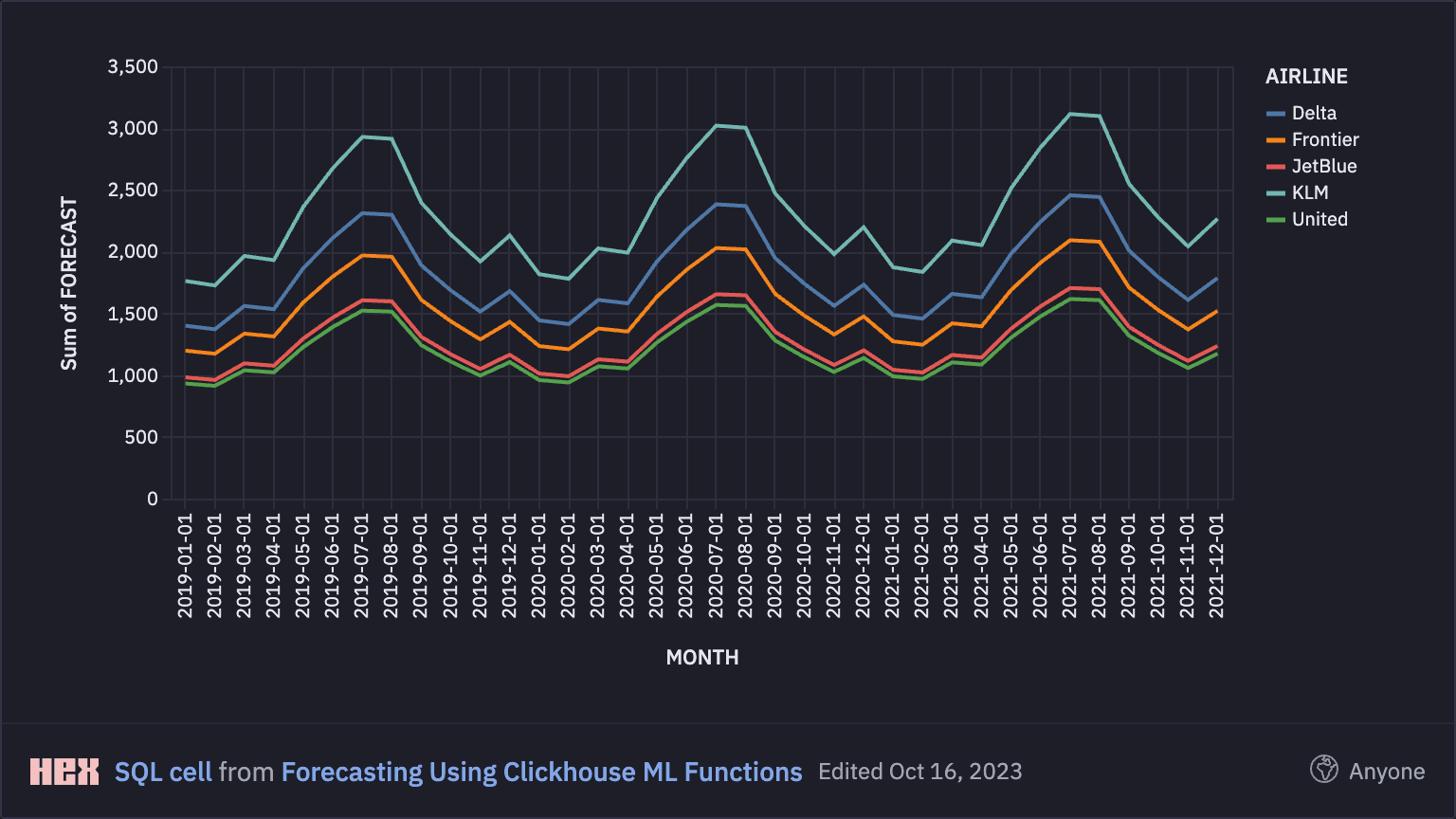
Giving us an end to end visualisation of this. Visually, we can see that the increase in passenger numbers and the seasonality has been captured by the out of range forecast.
Conclusion
In this article we have demonstrated how we can use the ML functions (stochasticLinearRegression and evalMLMethod) that are avaialable within ClickHouse to implement a simple forecasting technique.
In principle, offloading metrics and analytics work like this to the database is a good thing. An analytical database such as ClickHouse will generally outperform and allow us to work with datasets that are bigger than can be processed on a single machine, whilst also reducing the amount of scripting work that needs to take place.
In ClickHouse, this could also be built into a materialized view, meaning that models are continually updated and retrained as new data is captured opening up real-time possibilities.
We believe this pattern could grow in future, with more data science and machine learning algorithms being implemented directly within the database.
A notebook describing the full worked example can be found at this URL.