At ClickHouse, we often find ourselves downloading and exploring increasingly large datasets, which invariably need a fast internet connection. When looking to move house and country and needing to ensure I had fast internet, I discovered the sizable Ookla dataset providing internet performance for all locations around the world. This dataset represents the world's largest source of crowdsourced network tests, covering both fixed and mobile internet performance with coverage for the majority of the world's land surface.
While Ookla already provides excellent tooling for exploring internet performance by location using this dataset, it presented an opportunity to explore both ClickHouse's Apache Iceberg support as well as ever-expanding geo functions.
Limiting this a little further, I was curious to see the feasibility of visualizing geographical data with just SQL by converting geo polygons to SVGs. This takes us on a tour of h3 indexes, polygon dictionaries, Mercator projections, color interpolations, and centroid computation using UDFs. If you are curious how we ended up with the following with just SQL, read on…
Note: ClickHouse supports a number of visualization tools ideal for this dataset, including but not limited to Superset. Our limitation to using just SQL was just for fun!
Before diving into the dataset, we’ll do a quick refresh on the value of Apache Iceberg and its support and relevance to ClickHouse. For those familiar with this topic, feel free to jump to the part we start querying!
Apache Iceberg
Apache Iceberg has gathered significant attention in recent years, with it fundamental to the evolution of the “Data Lake” concept to a “Lake House.” By providing a high-performance table format for data, Iceberg brings table-like semantics to structured data stored in a data lake. More specifically, this open-table format is vendor-agnostic and allows data files, typically in structured Parquet, to be exposed as tables with support for schema evolution, deletes, updates, transactions, and even ACID compliance. This represents a logical evolution from more legacy data lakes based on technologies such as Hadoop and Hive.
Maybe, most importantly, this data format allows query engines like Spark and Trino to safely work with the same tables, at the same time, while also delivering features such as partitioning which potentially can be exploited by query planners to accelerate queries.
ClickHouse support
While ClickHouse is a lot more than simply a query engine, we acknowledge the importance of these open standards in allowing users to avoid vendor lock-in as well as a sensible data interchange format for other tooling. As discussed in a recent blog post, "The Unbundling of the Cloud Data Warehouse" we consider the lake house to be a fundamental component in the modern data architecture, complementing real-time analytical databases perfectly. In this architecture, the lake house provides cost-effective cold storage and a common source of truth, with support for ad hoc querying.
However, for more demanding use cases, such as user-facing data-intensive applications, which require low latency queries and support for high concurrency, subsets can be moved to ClickHouse. This allows users to benefit from both the open interchange format of Iceberg for their cold storage and long-term retention, using ClickHouse as a real-time data warehouse for when query performance is critical.

Querying Iceberg with ClickHouse
Realizing this vision requires the ability to query Iceberg files from ClickHouse. As a lake house format, this is currently supported through a dedicated table iceberg function. This assumes the data is hosted on an S3-compliant service such as AWS S3 or Minio.
For our examples, we’ve made the Ookla dataset available in the following public S3 bucket for users to experiment.
s3://datasets-documentation/ookla/iceberg/
We can describe the schema of the Ookla data using a DESCRIBE query with the iceberg function replacing our table name. Unlike Parquet, which relies on sampling the actual data, the schema is read from the Iceberg metadata files.
DESCRIBE TABLE iceberg('https://datasets-documentation.s3.eu-west-3.amazonaws.com/ookla/iceberg/')
SETTINGS describe_compact_output = 1

┌─name────────────┬─type─────────────┐
│ quadkey     	  │ Nullable(String) │
│ tile        	  │ Nullable(String) │
│ avg_d_kbps  	  │ Nullable(Int32)  │
│ avg_u_kbps  	  │ Nullable(Int32)  │
│ avg_lat_ms  	  │ Nullable(Int32)  │
│ avg_lat_down_ms │ Nullable(Int32)  │
│ avg_lat_up_ms   │ Nullable(Int32)  │
│ tests       	  │ Nullable(Int32)  │
│ devices     	  │ Nullable(Int32)  │
│ year_month  	  │ Nullable(Date)   │
└─────────────────┴──────────────────┘

10 rows in set. Elapsed: 0.216 sec.
Similarly, querying rows can be performed with standard SQL with the table function replacing the table name. In the following, we sample some rows and count the total size of the data set.
SELECT *
FROM iceberg('https://datasets-documentation.s3.eu-west-3.amazonaws.com/ookla/iceberg/')
LIMIT 1
FORMAT Vertical

Row 1:
──────
quadkey:     	1202021303331311
tile:        	POLYGON((4.9163818359375 51.2206474303833, 4.921875 51.2206474303833, 4.921875 51.2172068072334, 4.9163818359375 51.2172068072334, 4.9163818359375 51.2206474303833))
avg_d_kbps:  	109291
avg_u_kbps:  	15426
avg_lat_ms:  	12
avg_lat_down_ms: ᴺᵁᴸᴸ
avg_lat_up_ms:   ᴺᵁᴸᴸ
tests:       	6
devices:     	4
year_month:  	2021-06-01

1 row in set. Elapsed: 2.100 sec. Processed 8.19 thousand rows, 232.12 KB (3.90 thousand rows/s., 110.52 KB/s.)
Peak memory usage: 4.09 MiB.


SELECT count()
FROM iceberg('https://datasets-documentation.s3.eu-west-3.amazonaws.com/ookla/iceberg/')

┌───count()─┐
│ 128006990 │
└───────────┘

1 row in set. Elapsed: 0.701 sec. Processed 128.01 million rows, 21.55 KB (182.68 million rows/s., 30.75 KB/s.)
Peak memory usage: 4.09 MiB
We can see that Ookla divides the surface of the earth into Polygons using the WKT format. We’ll delve into this in the 2nd half of the blog; for now, we’ll complete our simple examples with an aggregation computing the average number of devices per polygon and the median, 90th, 99th, and 99.9th quantiles for download speed.
SELECT
    round(avg(devices), 2) AS avg_devices,
    arrayMap(m -> round(m / 1000), quantiles(0.5, 0.9, 0.99, 0.999)(avg_d_kbps)) AS download_mbps
FROM iceberg('https://datasets-documentation.s3.eu-west-3.amazonaws.com/ookla/iceberg/')

┌─avg_devices─┬─download_mbps────┐
│   	 5.64 │ [51,249,502,762] │
└─────────────┴──────────────────┘

1 row in set. Elapsed: 4.704 sec. Processed 128.01 million rows, 3.75 GB (27.21 million rows/s., 797.63 MB/s.)
Peak memory usage: 22.89 MiB.
The above provides some simple examples of how their real-time data warehouse might function: cold Iceberg storage in the lake house and hot queries for real-time analytics in ClickHouse.
A few limitations
The above represents some very simple queries. Before we dive into a deeper topic of how to visualize this data, it's worth highlighting some of the areas where further improvement is required (and planned) for ClickHouse's Iceberg support.
- Currently, ClickHouse will not read Iceberg files that have row-based deletes (v2) or whose schema has evolved. The user will receive a read exception in these cases unless they explicitly request it is ignored.
- During query evaluation, ClickHouse doesn't currently exploit partitions to prune the data scanned. This represents a significant possibility for improving query execution and aligns with the recent improvements made to Parquet.
- The current implementation is bound to S3. In the future, we expect this coupling to be removed, with support added for any object storage supported by ClickHouse.
- Similar to ClickHouse's ordering key, Iceberg supports the ability to sort data. By ensuring data files within the Iceberg table are split and sorted, queries can potentially skip files during execution. This has the potential to further reduce the data scanned, improving performance.
Exploring the data
With the basics out of the way, let's pivot this blog slightly and explore the Ookla data in a little more detail with the objective of visualizing internet speeds with just SQL.
Reading and enriching
As noted earlier, the Ookla data separates the earth into polygons of varying sizes from which internet performance statistics have been collected. These Polygons are defined in the WKT format, a markup language for representing spatial objects. This format makes sense for Iceberg and for data distribution purposes since the underlying Parquet files have no native Polygon representation.
POLYGON((-160.02685546875 70.6435894914449, -160.021362304688 70.6435894914449, -160.021362304688 70.6417687358462, -160.02685546875 70.6417687358462, -160.02685546875 70.6435894914449))
Querying this, however, requires conversion to a numerical representation. For ClickHouse, this can be performed with the readWKTPolygon function. As shown below, this converts the text representation to a Polygon type on which we can later use ClickHouse’s large range of geometric functions. Note these Polygons contain longitude and latitude values.
SELECT readWKTPolygon(assumeNotNull(tile)) AS poly, toTypeName(poly) as type
FROM iceberg('https://datasets-documentation.s3.eu-west-3.amazonaws.com/ookla/iceberg/')
LIMIT 1
FORMAT Vertical

Row 1:
──────
poly:                                        	[[(4.9163818359375,51.2206474303833),(4.921875,51.2206474303833),(4.921875,51.2172068072334),(4.9163818359375,51.2172068072334),(4.9163818359375,51.2206474303833)]]
type: Polygon

1 row in set. Elapsed: 1.920 sec. Processed 8.19 thousand rows, 232.12 KB (4.27 thousand rows/s., 120.91 KB/s.)
Peak memory usage: 4.10 MiB.
For a gentle introduction to Polygons and parsing WKT data, we recommend the following video from our very own “Data with Mark”.
Note the above video uses the most recent files from the Ookla dataset for which a centroid is provided.
While more recent versions of the Ookla dataset include a precomputed centroid of each polygon (from the 2nd quarter of 2023), the dataset goes back to 2019. As we’ll show later, this centroid (a lat/lon pair) can be useful when rendering the data. Fortunately, this is relatively simple to compute as our polygons are non-self-intersecting and closed. For the curious reader, some sample Python code (credit) is shown below.
def centroid(vertices):
	x, y = 0, 0
	n = len(vertices)
	signed_area = 0
       # computes the signed area and y and x accumulators - signed_area UDF function
	for i in range(len(vertices)):
    	  x0, y0 = vertices[i]
    	  x1, y1 = vertices[(i + 1) % n]
    	  # shoelace formula - maps to area function below
    	  area = (x0 * y1) - (x1 * y0)
    	  signed_area += area
    	  x += (x0 + x1) * area
    	  y += (y0 + y1) * area
       # final step of centroid function
	signed_area *= 0.5
	x /= 6 * signed_area
	y /= 6 * signed_area
	return x, y

x, y = centroid([(-160.037841796875, 70.6363054807905), (-160.032348632812, 70.6363054807905),(-160.032348632812, 70.6344840663086), (-160.037841796875, 70.6344840663086), (-160.037841796875, 70.6363054807905)])
print(x,y)
python centroid.py
-160.03509089358298 70.63539286610323
Converting this to a SQL UDF we can use at query time is simplest if we decompose the problem into several functions.
CREATE FUNCTION area AS (v1,v2) -> ((v1.1 * v2.2) - (v2.1 * v1.2))

CREATE FUNCTION signed_area AS polygon ->
   (
       arrayFold((acc, x) -> (
       (acc.1) + ((((x.1).1) + ((polygon[((x.2) + 1) % (length(polygon) + 1)]).1)) * area(x.1, polygon[((x.2) + 1) % (length(polygon) + 1)])),
       (acc.2) + ((((x.1).2) + ((polygon[((x.2) + 1) % (length(polygon) + 1)]).2)) * area(x.1, polygon[((x.2) + 1) % (length(polygon) + 1)])),
       (acc.3) + area(x.1, polygon[((x.2) + 1) % (length(polygon) + 1)])), arrayZip(polygon, range(1, length(polygon) + 1)), (0.0, 0.0, 0.0)
   )
)

CREATE FUNCTION centroid as polygon -> ((signed_area(polygon).1) / ((6 * (signed_area(polygon).3)) * 0.5), (signed_area(polygon).2) / ((6 * (signed_area(polygon).3)) * 0.5))
A quick test confirms our UDF gives the same result as the Python implementation.
SELECT centroid([(-160.037841796875, 70.6363054807905), (-160.032348632812, 70.6363054807905), (-160.032348632812, 70.6344840663086), (-160.037841796875, 70.6344840663086), (-160.037841796875, 70.6363054807905)]) AS centroid

┌─centroid────────────────────────────────┐
│ (-160.03509089358298,70.63539286610323) │
└─────────────────────────────────────────┘

1 row in set. Elapsed: 0.017 sec.
With the above functions, we can now read our Polygon data and compute a centroid consisting of a longitude and latitude. As we’ll show, we can exploit these centroids when visualizing the data.
Loading the data
While all of the following queries could be used with the iceberg table function, this requires the data to be downloaded for each query, often limiting performance to our network bandwidth. Since we're going to be running a number of queries, it makes sense to load the data into ClickHouse to enjoy the performance benefits highlighted earlier. We modify our table schema to include the converted Polygon (a Ring type - see below) and centroid (a Point type), extracting these with our functions above.
CREATE TABLE default.ookla
(
	`quadkey` Nullable(String),
	`polygon` Ring,
	`centroid` Point,
	`avg_d_kbps` Nullable(Int32),
	`avg_u_kbps` Nullable(Int32),
	`avg_lat_ms` Nullable(Int32),
	`avg_lat_down_ms` Nullable(Int32),
	`avg_lat_up_ms` Nullable(Int32),
	`tests` Nullable(Int32),
	`devices` Nullable(Int32),
	`year_month` Nullable(Date)
)
ENGINE = MergeTree ORDER BY tuple()

INSERT INTO ookla SELECT
	quadkey,
	readWKTPolygon(assumeNotNull(tile))[1] AS polygon,
	centroid(polygon) AS centroid,
	avg_d_kbps,
	avg_u_kbps,
	avg_lat_ms,
	avg_lat_down_ms,
	avg_lat_up_ms,
	tests,
	devices,
	year_month
FROM iceberg('https://datasets-documentation.s3.eu-west-3.amazonaws.com/ookla/iceberg/')

0 rows in set. Elapsed: 549.829 sec. Processed 128.01 million rows, 3.75 GB (232.81 thousand rows/s., 6.82 MB/s.)
Peak memory usage: 2.16 GiB.
Readers may notice that we use the first element from the array returned by the readWKTPolygon function. Polygons can consist of multiple rings, each consisting of a closed space. The first entry describes the outer space, with subsequent array entries specifying any holes. Since our polygons are closed, with no internal holes, we only have a single entry - allowing us to map our polygons to the simpler Ring type.
Our example only includes data for fixed devices. Data for mobile devices also exists for the curious.
Polygons to SVGs
As noted, we could exploit several visualization tools to render this data now. However, these do incur an overhead - installation and, more importantly, time to gain familiarity and expertise. Given that the SVG format is inherently a vector-based format capable of rendering polygons, maybe we can just convert these polygons to an SVG to provide a 2D visualization of the data as a map?
This requires a means of converting each polygon to an SVG polygon entry. Ideally, we’d also be able to set the style of each polygon to convey a metric, e.g., download speed. As ever, the community had already thought of this problem with ClickHouse providing the SVG function!
This allows us to convert a Polygon in ClickHouse to an SVG polygon, as well as passing a style:
SELECT SVG([(-160.037841796875, 70.6363054807905), (-160.032348632812, 70.6363054807905), (-160.032348632812, 70.6344840663086), (-160.037841796875, 70.6344840663086), (-160.037841796875, 70.6363054807905)], 'fill: rgb(255, 55,38);') AS svg FORMAT Vertical

Row 1:
──────
svg: <polygon points="-160.038,70.6363 -160.032,70.6363 -160.032,70.6345 -160.038,70.6345 -160.038,70.6363" style="fill: rgb(255, 55,38);"/>

1 row in set. Elapsed: 0.002 sec.
Points to Pixels
While the above is promising, we can't simply use coordinates as our latitudes and longitudes if visualizing as a 2d map. The coordinates represent positions on a three-dimensional surface, i.e., the Earth's surface, and not a 2d surface. A number of techniques, known as projections, exist for converting latitude and longitudes to points on 2d surfaces such as a map or a computer screen. This process inevitably involves some compromise or distortion in the representation of the Earth's surface because it's impossible to flatten a sphere without stretching or compressing its surface in some way.
A popular projection often used for maps is the Mercator projector. This has a number of advantages; principally, it preserves angles and shapes at a local scale, making it an excellent choice for navigation. It also has the advantage that constant bearings (directions of travel) are straight lines, making navigating simple. Finally, while the Mercator projection accurately represents areas near the equator, it significantly distorts size and shape as one moves toward the poles. Landmasses like Greenland and Antarctica appear much larger than they are in reality compared to equatorial regions.
While ClickHouse doesn't have a Mercator function built in, we can solve this with another SQL UDF. Here, we project our point into a pixel space with dimensions 1024x1024.
-- coord (lon, lat) format
CREATE OR REPLACE FUNCTION mercator AS (coord, width, height) -> (
   ((coord.1) + 180) * (width / 360),
   (height / 2) - ((width * ln(tan((pi() / 4) + ((((coord.2) * pi()) / 180) / 2)))) / (2 * pi()))
)

SELECT mercator((-160.037841796875, 70.6363054807905), 1024, 1024) AS pixel_coords

┌─pixel_coords──────────────────┐
│ (56.78125,223.79687511938704) │
└───────────────────────────────┘

1 row in set. Elapsed: 0.001 sec.
To apply the projection to an entire polygon, we can exploit the arrayMap function.
SELECT polygon, arrayMap(p -> mercator(p, 1024, 1024), polygon) AS pixels
FROM ookla
LIMIT 1
FORMAT Vertical

Row 1:
──────
polygon: [(-51.30615234375,-30.0358110426678),(-51.3006591796875,-30.0358110426678),(-51.3006591796875,-30.0405664305846),(-51.30615234375,-30.0405664305846),(-51.30615234375,-30.0358110426678)]
pixels:  [(366.0625,601.6406251005949),(366.078125,601.6406251005949),(366.078125,601.6562501003996),(366.0625,601.6562501003996),(366.0625,601.6406251005949)]

1 row in set. Elapsed: 0.012 sec.
Size limitations
With our SVG and Mercator functions, we are well-placed to generate our first SVG. The following query iterates over the full 128 million polygons and converts them to an svg element. We also output an opening and closing <svg> tag containing a background color and the coordinates for the viewBox.
For this initial query, we want to confirm this rendering technique works, and hence, use a fixed style and don’t consider any metrics for now. We redirect the output of this query to a file. Note we use the output format CustomSeparated to generate our svg opening and closing tag.
clickhouse client --query "SELECT SVG(arrayMap(p -> mercator(p, 1024, 1024), polygon), 'fill: rgb(255, 55,38);')
FROM ookla
FORMAT CustomSeparated
SETTINGS format_custom_result_before_delimiter = '<svg style=\"background-color: rgb(17,17,17);\" viewBox=\"0 0 1024 1024\" xmlns:svg=\"http://www.w3.org/2000/svg\" xmlns=\"http://www.w3.org/2000/svg\">', format_custom_result_after_delimiter = '</svg>', format_custom_escaping_rule = 'Raw'" > world.svg
What may have been predictable for many, is that 128 million polygons produce quite a large svg file!
(base) clickhouse@ClickHouse-MacBook-Pro ookla % ls -lh world.svg
-rw-r--r--  1 dalemcdiarmid  wheel	31G  2 Feb 17:04 world.svg
At 31GB, this isn’t renderable by a browser or tool on most machines and is even unrealistic to convert to compressed formats using tools such as ImageMagick. We welcome suggestions if you have an idea how to achieve this!
Summarizing using dictionaries
Our first effort might be to summarize the data into much larger polygons representing geographical regions. For this, we require a means of determining in which larger polygons our small polygons lie. This is possible with functions such as polygonsWithinCartesian, which will be expensive to compute for 128 million polygons.
Fortunately, ClickHouse has Polygon Dictionaries to address this very problem. These allow users to search for the polygon containing a specific point efficiently. This requires each of our small polygons to be represented by a single point, such as a centroid :)
As an example, suppose we want to summarize our polygons into countries. We store our target polygons in a countries table:
CREATE TABLE countries
(
  `name` String,
  `coordinates` MultiPolygon
)
ENGINE = MergeTree
ORDER BY name

INSERT INTO countries
SELECT name, coordinates
FROM (
SELECT JSONExtractString(JSONExtractString(json, 'properties'), 'ADMIN') as name,
JSONExtractString(JSONExtractRaw(json, 'geometry'), 'type') as type,
if(type == 'Polygon', [JSONExtract(JSONExtractRaw(JSONExtractRaw(json, 'geometry'), 'coordinates'), 'Polygon')], JSONExtract(JSONExtractRaw(JSONExtractRaw(json, 'geometry'), 'coordinates'), 'MultiPolygon')) as coordinates
 	FROM (SELECT arrayJoin(JSONExtractArrayRaw(json, 'features')) as json
       	FROM url('https://datasets-documentation.s3.eu-west-3.amazonaws.com/countries/countries.geojson', JSONAsString)))
Our country's polygons are represented as geoJSON and are available here. The above INSERT SELECT extracts these polygons from the JSON using JSONExtract* functions, storing them in the countries table.
And yet again we have a video for this very topic covering the query and subsequent dictionary:
CREATE DICTIONARY country_polygons
(
    `coordinates` MultiPolygon,
    `name` String
)
PRIMARY KEY coordinates
SOURCE(CLICKHOUSE(TABLE 'countries'))
LIFETIME(MIN 0 MAX 0)
LAYOUT(POLYGON(STORE_POLYGON_KEY_COLUMN 1))
This dictionary is indexed by the coordinates of our polygon and allows us to retrieve the polygon associated with a specific latitude and longitude using the dictGet function. For example,
SELECT dictGet(country_polygons, 'name', (-2.72647, 55.599621)) AS location

┌─location───────┐
│ United Kingdom │
└────────────────┘
1 row in set. Elapsed: 0.012 sec.
Notice the speed of retrieval here. Aside from being useful in our later visualizations, this dictionary allows us to obtain quick insight into the internet speeds of different countries. For example, we can quickly determine that maybe the South Georgia islands are the best place to live for fast internet!
SELECT dictGet(country_polygons, 'name', centroid) AS country,
    avg(avg_d_kbps) AS download_speed,
    sum(devices) AS total_devices
FROM ookla
GROUP BY country
ORDER BY download_speed DESC
LIMIT 10

┌─country──────────────────────────────────┬─────download_speed─┬─total_devices─┐
│ South Georgia and South Sandwich Islands │    		 198885 │    		 4  │
│ Singapore                       		   │ 197264.31481017102 │  	    3591446 │
│ Hong Kong S.A.R.                		   │   166375.523948868 │  	    3891226 │
│ China                           		   │ 158978.10242450528 │ 	   53841880 │
│ Thailand                        		   │ 155309.49656953348 │ 	   27506456 │
│ Iceland                         		   │ 152290.62935414084 │   	 281514 │
│ United States of America        		   │ 149532.95964270137 │     246966470 │
│ South Korea                     		   │  149115.5647068738 │  	    2129690 │
│ United Arab Emirates            		   │  148936.4285346194 │  	    8380900 │
│ Jersey                          		   │ 146030.67963711882 │   	 100902 │
└──────────────────────────────────────────┴────────────────────┴───────────────┘

10 rows in set. Elapsed: 5.467 sec. Processed 256.01 million rows, 6.66 GB (46.83 million rows/s., 1.22 GB/s.)
Peak memory usage: 129.74 MiB.
Finally, as we’ll see below, it might also be helpful to be able to retrieve the polygon for a country efficiently based on its name. This can be achieved with a simple dictionary using the same countries table.
CREATE DICTIONARY default.country_names
(
	`coordinates` MultiPolygon,
	`name` String
)
PRIMARY KEY name
SOURCE(CLICKHOUSE(TABLE 'countries'))
LIFETIME(MIN 0 MAX 0)
LAYOUT(COMPLEX_KEY_HASHED())

SELECT dictGet(country_names, 'coordinates', 'Yemen') AS coords

[[[(53.308239457000155,12.11839453700017),(53.310267307000146,12.11144367200015)..

1 row in set. Elapsed: 0.007 sec.
For more details on dictionaries we recommend the following blog post.
Global SVG
Armed with our dictionaries, centroids, Mercator UDF, and SVG functions, we can generate our first (usable) SVG.
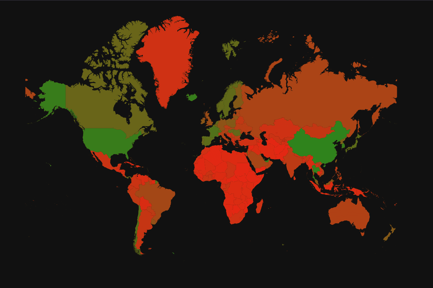
The above SVG is 9.2MB and is generated by the following query, which completes in 11 seconds. As shown in the key, red here represents slow internet speed (download rate), while green represents faster connection speed.
WITH
   -- settings determining height, width and color range
   1024 AS height, 1024 AS width, [234, 36, 19] AS lc, [0, 156, 31] AS uc,
   country_rates AS
   (
       -- compute the average download speed per country using country_polygons dictionary
       SELECT
           dictGet(country_polygons, 'name', centroid) AS country,
           avg(avg_d_kbps) AS download_speed
       FROM ookla
       -- exclude 'Antarctica' as polygon isnt fully closed
       WHERE country != 'Antarctica'
       GROUP BY country
   ),
   (
       -- compute min speed over all countries
       SELECT min(download_speed)
       FROM country_rates
   ) AS min_speed,
   (
       -- compute max speed over all countries
       SELECT max(download_speed)
       FROM country_rates
   ) AS max_speed,
   country_colors AS
   (
       SELECT
           country,
           download_speed,
           (download_speed - min_speed) / (max_speed - min_speed) AS percent,
           -- compute a rgb value based on linear interolation between yellow and red
           format('rgb({},{},{})', toUInt8((lc[1]) + (percent * ((uc[1]) - (lc[1])))), toUInt8((lc[2]) + (percent * ((uc[2]) - (lc[2])))), toUInt8((lc[3]) + (percent * ((uc[3]) - (lc[3]))))) AS rgb,
           --  get polygon for country name and mercator project every point
           arrayMap(p -> arrayMap(r -> arrayMap(x -> mercator(x, width, height), r), p), dictGet(country_names, 'coordinates', country)) AS pixel_poly
       FROM country_rates
   )
-- convert country polygon to svg
SELECT SVG(pixel_poly, format('fill: {};', rgb))
FROM country_colors
-- send output to file
INTO OUTFILE 'countries.svg'
FORMAT CustomSeparated
SETTINGS format_custom_result_before_delimiter = '<svg style="background-color: rgb(17,17,17);" viewBox="0 0 1024 1024" xmlns:svg="http://www.w3.org/2000/svg" xmlns="http://www.w3.org/2000/svg">', format_custom_result_after_delimiter = '</svg>', format_custom_escaping_rule = 'Raw'

246 rows in set. Elapsed: 1.396 sec. Processed 384.02 million rows, 8.06 GB (275.15 million rows/s., 5.78 GB/s.)
Peak memory usage: 39.54 MiB.
Despite just assembling the above concepts, there is a lot going on here. We’ve commented on the SQL, which hopefully helps, but in summary:
- We declare constants such as the color gradient (lc = yellow, uc = red) and the image height in the first CTE.
- For each country, we use the
country_polygonsdictionary to compute the average speed, similar to our earlier query. - For the above values, we determine the maximum and minimum internet speeds. These are used to generate color for each country, using a simple linear interpolation between our color ranges.
- For each country, using its name, we use the reverse dictionary
country_namesto obtain the polygon. These polygons are complex, with many internal holes represented as Rings. We thus need to use nestedarrayMapfunctions to project them using the Mercator projection function. - Finally, we convert the project country polygons to SVG using the SVG function and RGB values. This is output to a local file using the INTO OUTFILE clause.
Summarizing using h3 indexes
While the above query proves the concept of rendering SVGs from our geographical data, it is too coarse in its summarization. Visualizing internet speeds by country is interesting but only slightly builds on the earlier query, which listed internet speeds by country.
We could aim to populate our country_polygons dictionary with larger polygons from public sources. However, this seems a little restrictive, and ideally, we would be able to generate our vectors by a specified resolution, which controls the same of the polygons we render.
H3 is a geographical indexing system developed by Uber, where the Earth's surface is divided into a grid of even hexagonal cells. This system is hierarchical, i.e., each hexagon on the top level ("parent") can be split into seven even smaller ones ("children"), and so on. When using the indexing system, we define a resolution between 0 and 15. The greater the resolution, the smaller each hexagon and, thus, the greater number required to cover the Earth's surface.
The differences in resolution on the number of polygons can be illustrated with a simple ClickHouse query using the function h3NumHexagons, which returns the number of hexagons per resolution.
SELECT h3NumHexagons(CAST(number, 'UInt8')) AS num_hexagons
FROM numbers(0, 16)

┌─res─┬────num_hexagons─┐
│   0 │    		    122 │
│   1 │    		    842 │
│   2 │   		   5882 │
│   3 │  		  41162 │
│   4 │ 		  88122 │
│   5 │		    2016842 │
│   6 │   	   14117882 │
│   7 │   	   98825162 │
│   8 │  	  691776122 │
│   9 │ 	 4842432842 │
│  10 │     33897029882 │
│  11 │    237279209162 │
│  12 │   1660954464122 │
│  13 │  11626681248842 │
│  14 │  81386768741882 │
│  15 │ 569707381193162 │
└─────┴─────────────────┘

16 rows in set. Elapsed: 0.001 sec.
ClickHouse supports h3 through a number of functions, including the ability to convert a longitude and latitude to a h3 index via the geoToH3 function with a specified resolution. Using this function, we can convert our centroids to a h3 index on which we can aggregate and compute statistics such as average download speed. Once aggregated, we can reverse this process with the function h3ToGeoBoundary to convert a h3 index and its hexagon to a polygon. Finally, we use this Mercator projection and SVG function to produce our SVG. We visualize this process below:
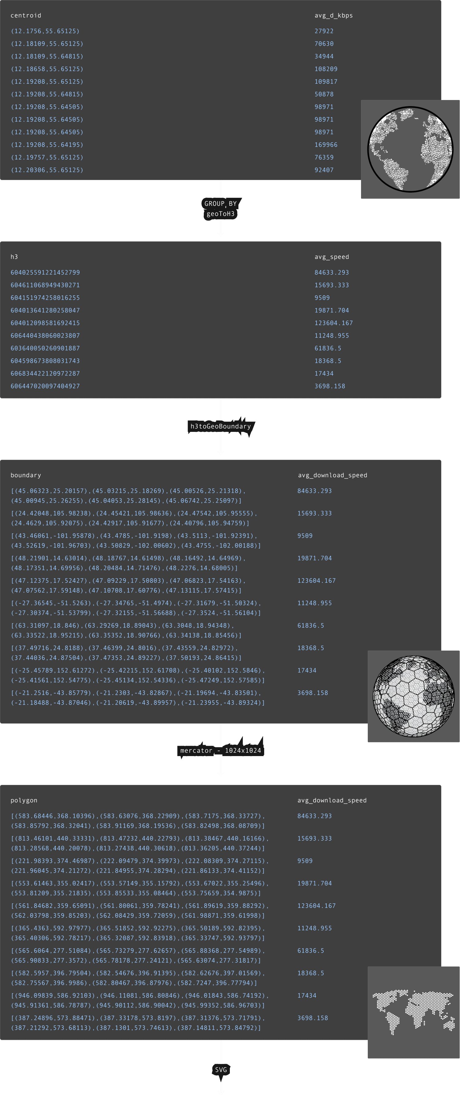
Above, we show the result for a resolution of 6, which produces 14,117,882 polygons and a file size of 165MB. This takes Chrome around 1 minute to render on a Macbook M2. By modifying the resolution, we can control the size of our polygons and the level of detail in our visualization. If we reduce the resolution to 4, our file size also decreases to 9.2MB as our visualization becomes more coarser with Chrome able to render this almost instantly.
Our query here:
Our query here:
WITH
   1024 AS height, 1024 AS width, 6 AS resolution, 30 AS lc, 144 AS uc,
   h3_rates AS
   (
       SELECT
           geoToH3(centroid.1, centroid.2, resolution) AS h3,
           avg(avg_d_kbps) AS download_speed
       FROM ookla
       – filter out as these are sporadic and don’t cover the continent
       WHERE dictGet(country_polygons, 'name', centroid) != 'Antarctica'
       GROUP BY h3
   ),
   (
       SELECT min(download_speed) FROM h3_rates
   ) AS min_speed,
   (
       SELECT quantile(0.95)(download_speed) FROM h3_rates
   ) AS max_speed,
   h3_colors AS
   (
       SELECT
           -- sqrt gradient
           arrayMap(x -> (x.2), arrayConcat(h3ToGeoBoundary(h3), [h3ToGeoBoundary(h3)[1]])) AS longs,
           sqrt(download_speed - min_speed) / sqrt(max_speed - min_speed) AS percent,
           -- oklch color with gradient on hue
           format('oklch(60% 0.23 {})', toUInt8(lc + (percent * (uc - lc)))) AS oklch,
           arrayMap(p -> mercator((p.2, p.1), width, height), h3ToGeoBoundary(h3)) AS pixel_poly
       FROM h3_rates
       -- filter out points crossing 180 meridian
       WHERE arrayExists(i -> (abs((longs[i]) - (longs[i + 1])) > 180), range(1, length(longs) + 1)) = 0
   )
SELECT SVG(pixel_poly, format('fill: {};', oklch))
FROM h3_colors
INTO OUTFILE 'h3_countries.svg' TRUNCATE
FORMAT CustomSeparated
SETTINGS format_custom_result_before_delimiter = '<svg style="background-color: rgb(17,17,17);" viewBox="0 0 1024 1024" xmlns:svg="http://www.w3.org/2000/svg" xmlns="http://www.w3.org/2000/svg">', format_custom_result_after_delimiter = '</svg>', format_custom_escaping_rule = 'Raw'

55889 rows in set. Elapsed: 10.101 sec. Processed 384.02 million rows, 8.06 GB (38.02 million rows/s., 798.38 MB/s.)
Peak memory usage: 23.73 MiB.
Aside from the conversion of the centroids to h3 indexes and their aggregation, there are a few other interesting parts of this query:
- We extract the longitudes into a separate array, and the first entry is also appended to the end. I.e.
arrayMap(x -> (x.2), arrayConcat(h3ToGeoBoundary(h3), [h3ToGeoBoundary(h3)[1]])). This allows us to examine consecutive pairs of longitudinal points and filter out those which cross the 180 meridian (these render as lines ruining our visual) i.e.WHERE arrayExists(i -> (abs((longs[i]) - (longs[i + 1])) > 180), range(1, length(longs) + 1)) = 0 - Rather than using an RGB color gradient, we’ve opted to use Oklch. This offers several advantages of RGB (and HSL), delivering more expected results and smoother gradients while being easier to generate as only one dimension (hue) needs to be changed for our palette. Above our palette goes from red (low bandwidth) to green (high bandwidth), with a square root gradient between 30 and 144 hues. The
sqrthere gives us a more even distribution of values, which are naturally clustered if linear, allowing us to differentiate regions. Our use of the 95th percentile for 144 also helps here.
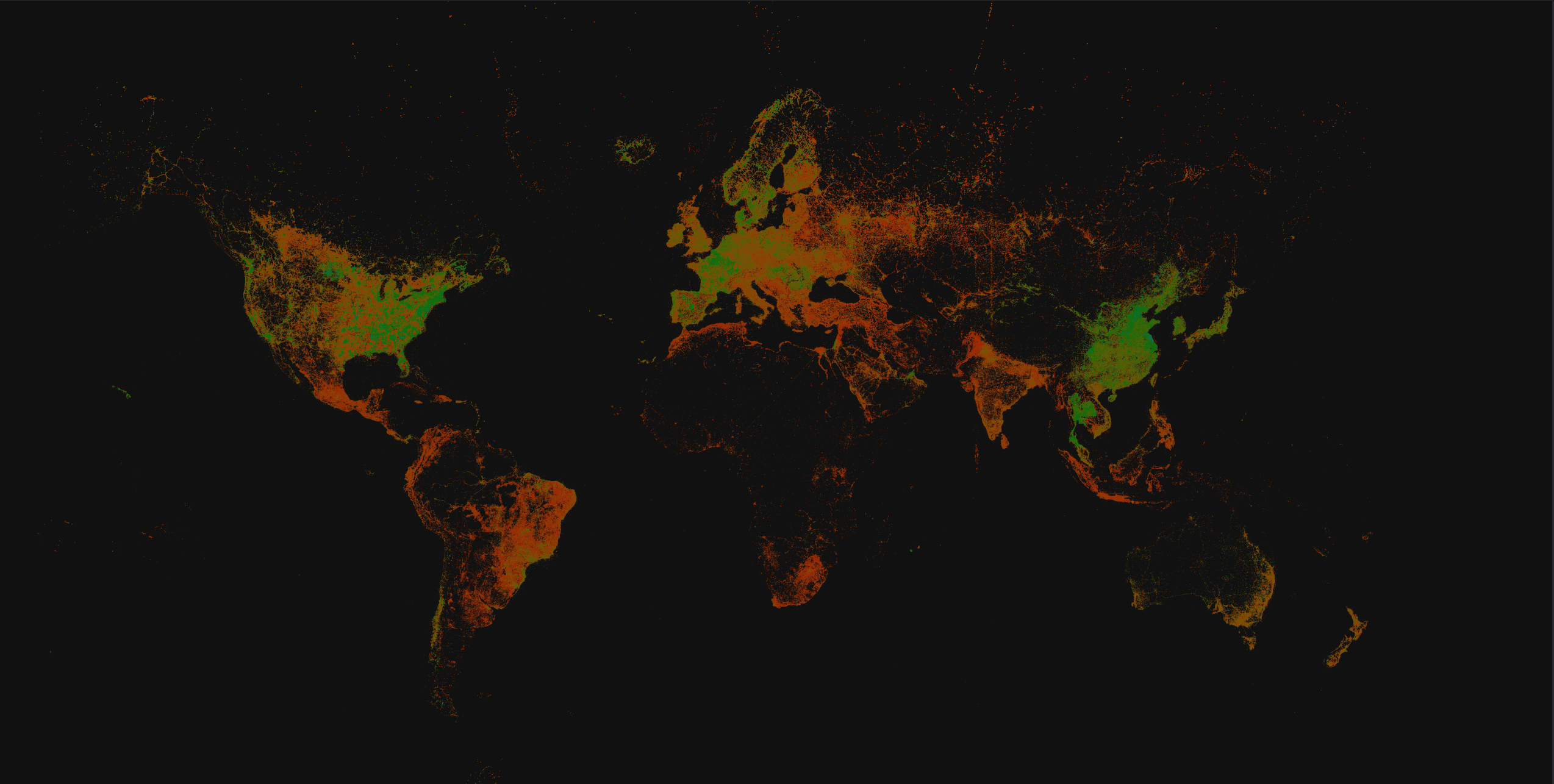
Rasterizing as an alternative
The h3 index approach above is flexible and realistic for rendering images based on a resolution of up to around 7. Values higher than this produce files that can’t be rendered by most browsers, e.g., 7 and 8 produce a file size of 600MB (just about renders!) and 1.85GB. The absence of data for some geographical regions (e.g. Africa) also becomes more apparent at these higher resolutions as the polygons for each centroid become smaller, i.e. more space is simply empty.
An alternative to this approach is to rasterize the image, generating a pixel for each centroid instead of a polygon. This approach is potentially also more flexible as when we specify the desired resolution (through the Mercator) function, this will map directly to the number of pixels used to represent our centroids. The data representation should also be smaller on disk for the same equivalent number of polygons.
The principle of this approach is simple. We project each centroid using our Mercator function, specifying a resolution and rounding the x and y values. Each of these x and y pairs represents a pixel, for which we can compute a statistic such as the average download rate using a simple GROUP BY. The following computes the average download rate per x,y pixel (for a resolution of 2048 x2048) using this approach, returning the pixels in row and column order.
SELECT
	(y * 2048) + x AS pos,
	avg(avg_d_kbps) AS download_speed
FROM ookla
GROUP BY
	round(mercator(centroid, 2048, 2048).1) AS x,
	round(mercator(centroid, 2048, 2048).2) AS y
ORDER BY pos ASC WITH FILL FROM 0 TO 2048 * 2048
Using the same approaches described above, the following query computes a color gradient using the min and max range of the download speed, outputting an RGBA value for each pixel. Below, we fix the alpha channel to 255 and use a linear function for our color gradient with the 95th percentile as our upper bound (to help compress our gradient). In this case, we use the query to create a view ookla_as_pixels to simplify the next step of visualizing this data. Note we use a background color of (17, 17, 17, 255) to represent those pixels with a null value for the download speed, i.e. no data points, and ensure our RGBA values are UInt8s.
CREATE OR REPLACE VIEW ookla_as_pixels AS
WITH [234, 36, 19] AS lc, [0, 156, 31] AS uc, [17,17,17] As bg,
pixels AS
(
	SELECT (y * 2048) + x AS pos,
    	avg(avg_d_kbps) AS download_speed
	FROM ookla
	GROUP BY
    	round(mercator(centroid, 2048, 2048).1) AS x,
    	round(mercator(centroid, 2048, 2048).2) AS y
	ORDER BY
    	pos WITH FILL FROM 0 TO 2048 * 2048
),
(
	SELECT min(download_speed)
	FROM pixels
) AS min_speed,
(
	SELECT quantile(0.95)(download_speed)
	FROM pixels
) AS max_speed,
pixel_colors AS (
	SELECT
	least(if(isNull(download_speed),0, (download_speed - min_speed) / (max_speed - min_speed)), 1.0) AS percent,
	if(isNull(download_speed),bg[1], toUInt8(lc[1] + (percent * (uc[1] - lc[1])))) AS red,
	if(isNull(download_speed),bg[2], toUInt8(lc[2] + (percent * (uc[2] - lc[2])))) AS green,
	if(isNull(download_speed),bg[3], toUInt8(lc[3] + (percent * (uc[3] - lc[3])))) AS blue
	FROM pixels
) SELECT red::UInt8, green::UInt8, blue::UInt8, 255::UInt8 as alpha FROM pixel_colors
Converting this data to an image is most easily done using a Canvas element and some simple js. We effectively have 4 bytes per pixel and 2048 x 2048 x 4 bytes in total or approximately 16MB. Using the putImageData we render this data directly into a canvas.
<!doctype html>
<html>
<head>
   <meta charset="utf-8">
   <link rel="icon" href="favicon.png">
   <title>Simple Ookla Visual</title>
</head>
<body>
   <div id="error"></div>
   <canvas id="canvas" width="2048" height="2048"></canvas>
   <script>
       async function render(tile) {
           const url = `http://localhost:8123/?user=default&default_format=RowBinary`;
           const response = await fetch(url, { method: 'POST', body: 'SELECT * FROM ookla_as_pixels' });
           if (!response.ok) {
               const text = await response.text();
               let err = document.getElementById('error');
               err.textContent = text;
               err.style.display = 'block';
               return;
           }
           buf = await response.arrayBuffer();
           let ctx = tile.getContext('2d');
           let image = ctx.createImageData(2048, 2048);
           let arr = new Uint8ClampedArray(buf);

           for (let i = 0; i < 2048 * 2048 * 4; ++i) {
               image.data[i] = arr[i];
           }
           ctx.putImageData(image, 0, 0, 0, 0, 2048, 2048);
           let err = document.getElementById('error');
           err.style.display = 'none';
       }
       const canvas = document.getElementById("canvas");
       render(canvas).then((err) => {
           if (err) {
               let err = document.getElementById('error');
               err.textContent = text;
           } else {
               err.style.display = 'none'
           }
       })
   </script>
</body>
</html>
This code provided by Alexey Milovidov who has taken this to a whole new level with his Interactive visualization and analytics on ADS-B data.
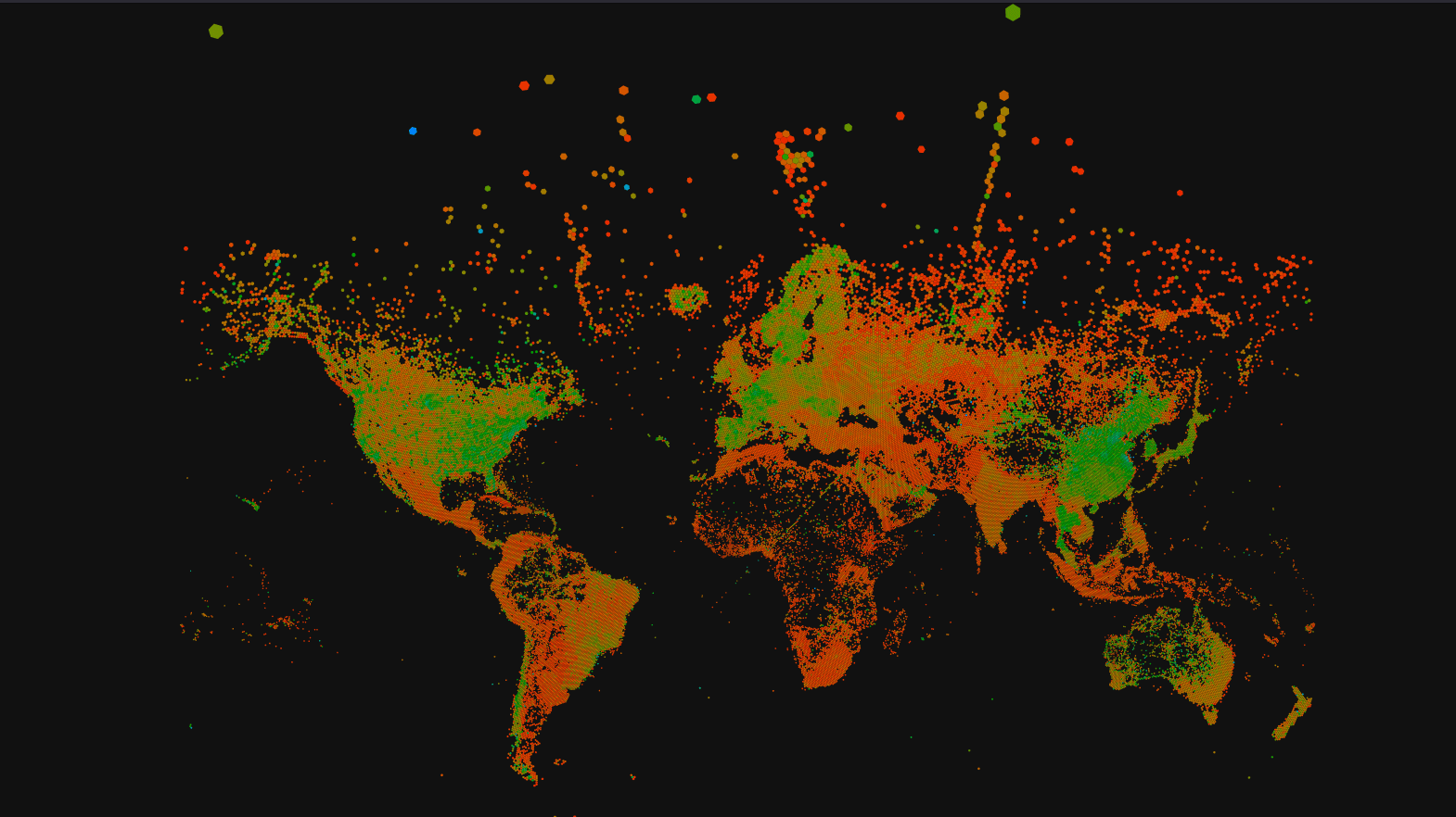
The above exploits the ClickHouse’s HTTP interface and ability to return results in RowBinary format. The creation of a view has significantly simplified our SQL query to simply SELECT * FROM ookla_as_pixels. Our resulting image.
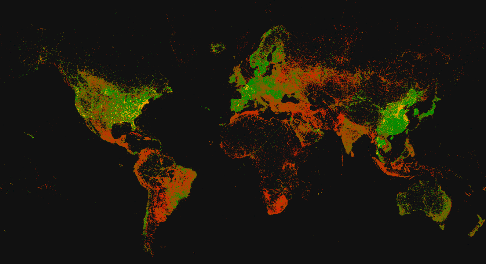
This represents a nice alternative to our SVG approach, even if we did have to use a little more than just SQL :)
Conclusion
This post has introduced the Iceberg data format and discussed the current state of support in ClickHouse, with examples of how to query and import the data. We have explored the Ookla internet speed dataset, distributed in Iceberg format, and used the opportunity to explore h3 indexes, polygon dictionaries, Mercator projections, color interpolations, and centroid computation using UDFs - all with the aim of visualizing the data with just SQL.
While we have mainly focused on download speed and fixed devices, we’d love to see others use similar approaches to explore other metrics. Alternatively, we welcome suggestions on improving the above!