Introduction
Operating any sophisticated technological stack in production without proper observability is analogous to flying an airplane without instruments. While it can work and pilots are trained for it, the risk/reward ratio is far from favorable and it should always be a last resort situation.

As the initial pillar of observability, centralized logging can be used for a wide variety of purposes: from debugging production incidents, resolving customer support tickets, mitigating security breaches, and even understanding how customers use the product.
The most important feature of any centralized log store is its ability to quickly aggregate, analyze, and search through vast amounts of log data from diverse sources. This centralization streamlines troubleshooting, making it easier to pinpoint the root causes of service disruptions. Look no further than Elastic, Datadog, and Splunk, who have leveraged this value proposition for huge success.
With users increasingly price-sensitive and finding the cost of these out-of-the-box offerings to be high and unpredictable in comparison to the value they bring, cost-efficient and predictable log storage, where query performance is acceptable, is more valuable than ever.
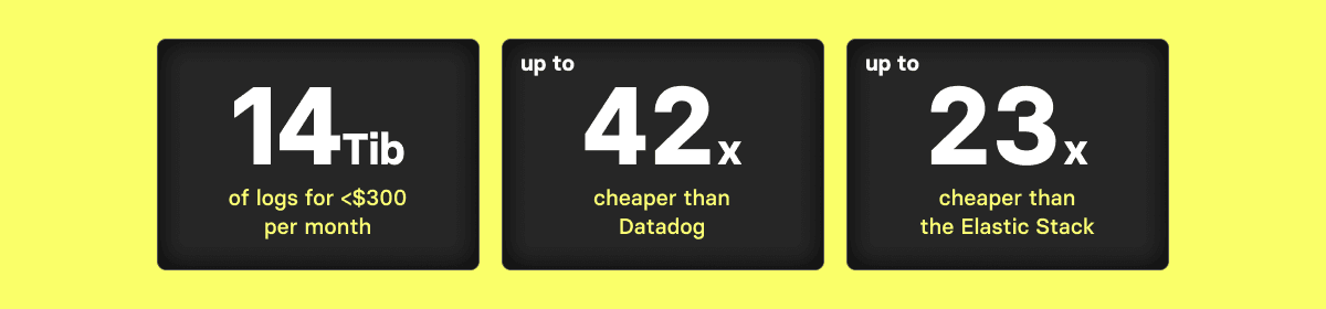
In this post, we introduce the CGW Stack (ClickHouse, Grafana, WarpStream or “Can’t Go Wrong”) and demonstrate how this offers compression rates over 10x for typical log data, when coupled with separation of storage and compute, allows a ClickHouse Cloud Development tier instance to comfortably host over 1.5TiB of log data (around 5 billion rows assuming a similar number of columns to our sample data): compressing this down to under 100GiB. A fully parallelized query execution engine, coupled with low-level optimizations, ensures query performance remains under 1s for most typical SRE queries on these volumes as demonstrated by our benchmark.
With compression rates of up to 14x in our benchmarks, this cluster (which allows up to 1TiB of compressed data) can potentially store up to 14 TiB of uncompressed log data. Users can either use this spare capacity to increase storage density even further if query performance is less critical or, alternatively, just use it to simply retain data for longer. We show the savings are dramatic in comparison to other solutions, such as Elastic and Datadog, which are between 23x and 42x more expensive for the same data volume.
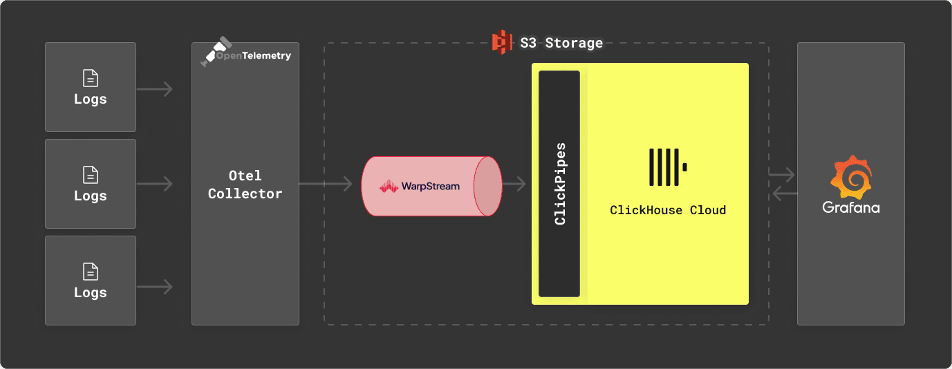
While ClickHouse can be used standalone as a log storage engine, we appreciate users often prefer an architecture in which data is first buffered in Kafka prior to its insertion into ClickHouse. This provides a number of benefits, principally the ability to absorb spikes in traffic whilst keeping the insertion load on ClickHouse constant and allowing data to be forwarded to other downstream systems. Looking to keep costs and operations as low as possible in our proposed architecture, we consider a Kafka implementation that also separates storage and compute: WarpStream. We combine this with our standard recommendations of OTEL for log collection and Grafana for visualization.
Why ClickHouse?
As a high-performance OLAP database, ClickHouse is used for many use cases, including real-time analytics for time series data. Its diversity of use cases has helped drive a huge range of analytical functions, which assist in querying most data types. These query features and very high compression rates, resulting from the column-oriented design and customizable codecs, have increasingly led users to choose ClickHouse as a log data store. By separating storage and compute, and utilizing object storage as its principal data store, ClickHouse Cloud further increases this cost efficiency.
While we have historically seen large CDN providers using ClickHouse for storage of logs, with the cost of logging solutions increasingly in the spotlight, we now increasingly see small and medium-sized businesses considering ClickHouse as a log storage alternative as well.
What is WarpStream?
WarpStream is an Apache Kafka® protocol compatible data streaming platform that runs directly on top of any commodity object-store. Like ClickHouse, WarpStream was designed from the ground up for analytical use cases and to help manage huge streams of machine-generated data as cost-effectively as possible.
Instead of Kafka brokers, WarpStream has “Agents”. Agents are stateless Go binaries (no JVM!) that speak the Kafka protocol, but unlike a traditional Kafka broker, any WarpStream Agent can act as the “leader” for any topic, commit offsets for any consumer group, or act as the coordinator for the cluster. No Agent is special, so auto-scaling them based on CPU usage or network bandwidth is trivial.
This is made possible by the fact that WarpStream separates both compute from storage and_ data from metadata.The_ metadata for every WarpStream “Virtual Cluster” is stored in a custom metadata database that was written from the ground up to solve this exact problem in the most performant and cost-effective way possible.
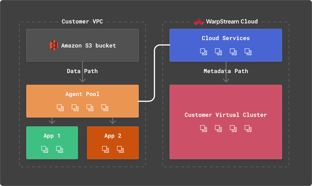
The fact that WarpStream uses object storage as the primary and only storage, with zero local disks, makes it excel with analytical data compared to other Apache Kafka implementations.
Specifically, WarpStream uses object storage as the storage layer and the network layer to avoid inter-az bandwidth costs entirely, whereas these fees can easily represent 80% of the total cost of a workload with traditional Apache Kafka implementations. In addition, the stateless nature of the Agents makes it practical (even easy) to scale workloads up to GiB/s of data.
These properties make WarpStream ideal for a logging solution where throughput volumes are often significant and price sensitivity is critical, and delivery latencies of a few seconds are more than acceptable.
For users looking to deploy a WarpStream for testing, you can follow these instructions to deploy a test cluster to Fly.io or these instructions to deploy on Railway.
ClickHouse Cloud Development tier
ClickHouse Cloud allows users to deploy ClickHouse with a separation of storage and compute. While users can control the CPU and memory assigned to a service for production tiers or allow it to automatically scale dynamically, the Development tier offers the ideal solution for our cost-efficient logging store. With a recommended limit of 1TiB for storage and compute limited to 4 CPUs and 16 GiB of memory, this instance type cannot exceed $193/month (assuming all 1TiB is used). For other use cases, the cost is typically lower than this due to the ability of the service to idle when not used. We assume the continuous nature of log ingestion means this isn’t viable. Despite this, this service is ideal for log storage for users needing to store up to 14TiB of raw log data, given the expected 14x compression ratio achieved by ClickHouse.
Note that the Development tier uses a reduced number of replica nodes to production instead - 2 instead of 3. This level of availability is also sufficient for Logging use cases where a replication factor of 2 is often sufficient to meet SLA requirements. Finally, the limited storage of TiB of compressed data allows a simple costing model to be developed, which we present below.
Example dataset
In order to benchmark a Development tier instance in ClickHouse Cloud for the logging use case, we require a representative dataset. For this, we use a publicly available Web Server Access Log dataset. While the schema of this dataset is simple, it is equivalent to commonly held nginx and Apache logs.
54.36.149.41 - - [22/Jan/2019:03:56:14 +0330] "GET /filter/27|13%20%D9%85%DA%AF%D8%A7%D9%BE%DB%8C%DA%A9%D8%B3%D9%84,27|%DA%A9%D9%85%D8%AA%D8%B1%20%D8%A7%D8%B2%205%20%D9%85%DA%AF%D8%A7%D9%BE%DB%8C%DA%A9%D8%B3%D9%84,p53 HTTP/1.1" 200 30577 "-" "Mozilla/5.0 (compatible; AhrefsBot/6.1; +http://ahrefs.com/robot/)" "-"
31.56.96.51 - - [22/Jan/2019:03:56:16 +0330] "GET /image/60844/productModel/200x200 HTTP/1.1" 200 5667 "https://www.zanbil.ir/m/filter/b113" "Mozilla/5.0 (Linux; Android 6.0; ALE-L21 Build/HuaweiALE-L21) AppleWebKit/537.36 (KHTML, like Gecko) Chrome/66.0.3359.158 Mobile Safari/537.36" "-"
31.56.96.51 - - [22/Jan/2019:03:56:16 +0330] "GET /image/61474/productModel/200x200 HTTP/1.1" 200 5379 "https://www.zanbil.ir/m/filter/b113" "Mozilla/5.0 (Linux; Android 6.0; ALE-L21 Build/HuaweiALE-L21) AppleWebKit/537.36 (KHTML, like Gecko) Chrome/66.0.3359.158 Mobile Safari/537.36" "-"
This 3.5GiB dataset contains around 10m log lines and covers 4 days in 2019. More importantly, the cardinality of the columns and cyclic patterns of the data are representative of real data. Utilizing a publicly available script, we have converted this dataset to CSV* to simplify insertion. The size of the respective files remains comparable. The resulting ClickHouse schema is shown below:
CREATE TABLE logs
(
  `remote_addr` String,
  `remote_user` String,
  `runtime` UInt64,
  `time_local` DateTime,
  `request_type` String,
  `request_path` String,
  `request_protocol` String,
  `status` UInt64,
  `size` UInt64,
  `referer` String,
  `user_agent` String
)
ENGINE = MergeTree
ORDER BY (toStartOfHour(time_local), status, request_path, remote_addr)
This represents a naive, non-optimized schema. Further optimizations are possible, which improve compression rates by 5% in our tests. However, the above represents a getting-started experience for a new user. We, therefore, test with the least favorable configuration. Alternative schemas can be found here, showing the changes in compression.
We have replicated this data to cover a one month period so we can project a more typical retention interval. While this causes the repetition of any inherent data patterns, this is considered sufficient for our tests and akin to typical weekly periodicity seen in logging use cases.
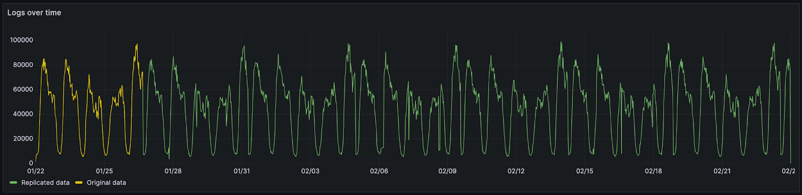
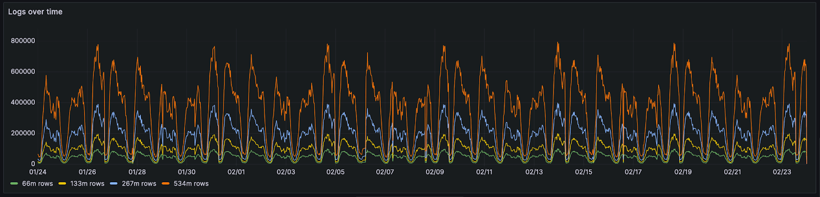
This month's data consists of 66 million rows and 20GiB of raw CSV/log data. In order to replicate this data for larger tests and preserve its data properties, we use a simple technique. Rather than simply duplicate data, we merge the existing data with a copy whose order has been randomized. This involves a simple script that iterates through both authoritative and randomized files line by line. Lines from the randomized and authoritative files are copied into a target file. Both "paired lines" are assigned the date from the authoritative file. This ensures the cyclic pattern shown above is preserved. This is in contrast to simply duplicating lines, which would cause duplicate lines to be placed next to each other. This would benefit compression and provide an unfair comparison - worsening as we duplicated the data. Below, we show the same data duplicated using the above technique for 133 million, 534 million, and a billion log lines.
 *In a production scenario we would recommend using a collector such as OTEL for this.
Loading log data with ClickPipes - data pipelines in less than a minute
All files used for our benchmark are available in the S3 bucket s3://datasets-documentation/http_logs/ for download and to allow users to replicate tests. This data is in CSV format for convenience. For users looking to load this data into a representative environment, we provide the following utility. This pushes data to a WarpStream instance, as shown below.
clickpipes -broker $BOOTSTRAP_URL -username $SASL_USERNAME -password $SASL_PASSWORD -topic $TOPIC -file data-66.csv.gz
wrote 0 records in 3.5µs, rows/s: 0.000000
generated schema: [time_local remote_addr remote_user runtime request_type request_path request_protocol status size referer user_agent]
wrote 10000 records in 63.2115ms, rows/s: 158198.854156
wrote 20000 records in 1.00043025s, rows/s: 19991.397861
wrote 30000 records in 2.000464333s, rows/s: 14996.517996
wrote 40000 records in 3.000462042s, rows/s: 13331.279947
wrote 50000 records in 4.000462s, rows/s: 12498.556286
To consume this data from WarpStream, users can, in turn, use ClickPipes, ClickHouse Cloud's native ingestion tool, to insert this data into ClickHouse. We demonstrate this below.
For users looking to only perform testing of ClickHouse, sample data files can be loaded from the ClickHouse client with a single command, as shown below.
INSERT INTO logs FROM INFILE 'data-66.csv.gz' FORMAT CSVWithNames
Compression
To evaluate the storage efficiency of ClickHouse, we show the uncompressed and compressed size of tables with increasing numbers of log events for the above dataset. The uncompressed size here can be considered analogous to the raw data volume in CSV or raw log format (although it's a little less).
SELECT
	table,
	formatReadableQuantity(sum(rows)) AS total_rows,
	formatReadableSize(sum(data_compressed_bytes)) AS compressed_size,
	formatReadableSize(sum(data_uncompressed_bytes)) AS uncompressed_size,
	round(sum(data_uncompressed_bytes) / sum(data_compressed_bytes), 2) AS ratio
FROM system.parts
WHERE (table LIKE 'logs%') AND active
GROUP BY table
ORDER BY sum(rows) ASC

┌─table─────┬─total_rows─────┬─compressed_size─┬─uncompressed_size─┬─ratio─┐
│ logs_66   │ 66.75 million  │ 1.27 GiB    	   │ 18.98 GiB     	   │ 14.93 │
│ logs_133  │ 133.49 million │ 2.67 GiB    	   │ 37.96 GiB     	   │ 14.21 │
│ logs_267  │ 266.99 million │ 5.42 GiB    	   │ 75.92 GiB     	   │	14 │
│ logs_534  │ 533.98 million │ 10.68 GiB   	   │ 151.84 GiB    	   │ 14.22 │
│ logs_1068 │ 1.07 billion   │ 20.73 GiB   	   │ 303.67 GiB    	   │ 14.65 │
│ logs_5340 │ 5.34 billion   │ 93.24 GiB   	   │ 1.48 TiB      	   │ 16.28 │
└───────────┴────────────────┴─────────────────┴───────────────────┴───────┘
Our compression ratio of approximately 14x remains constant, irrespective of the data volume. Our largest dataset, containing over 5b rows and 1.5TiB of uncompressed data, has a higher compression rate. We attribute this to greater duplication in the data as a result of the initially limited sample size of 10m rows. Note that the total size of data on disk can be improved by around 5% with further schema optimizations.
Importantly, even our largest dataset consumes less than 10% of the storage of our Development service at less than 100GiB. Users could retain ten months of data if desired at a minimal cost increase (see Cost analysis below).
Visualizing log data
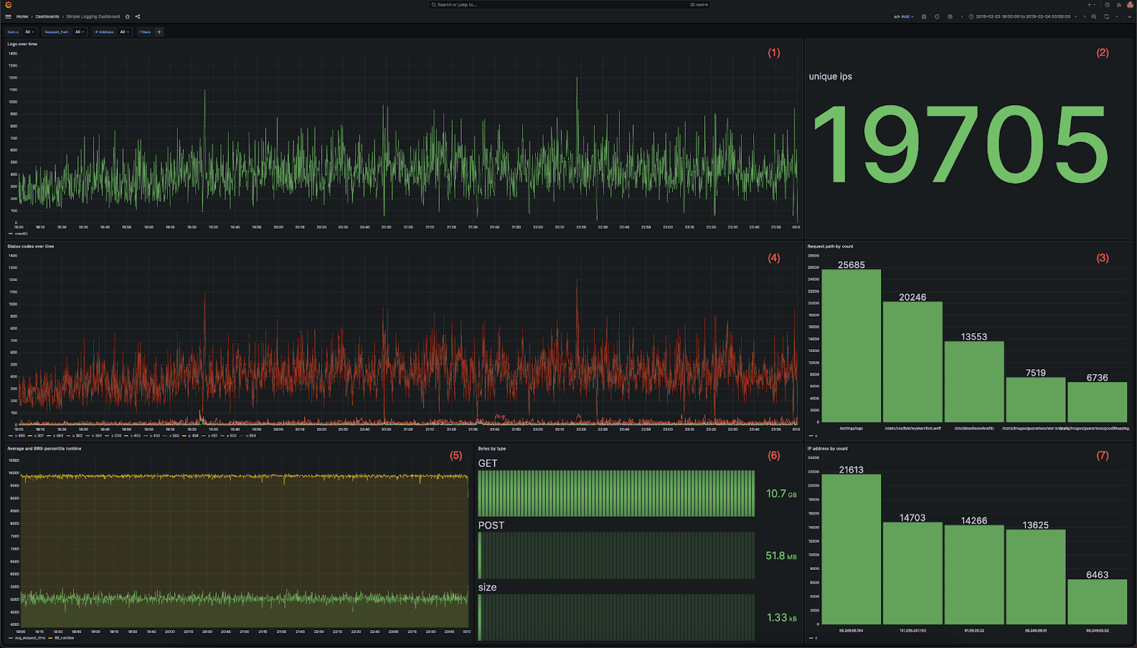
For visualization, we recommend using Grafana and the official ClickHouse plugin. In order to benchmark ClickHouse performance under a representative query load, we utilize the following dashboard. This contains 7 visualizations, each using a mixture of aggregations:
- A line chart showing logs over time
- A metric showing the total IPs inbound IP addresses
- A bar chart showing the top 5 website paths accessed
- Status codes over time as a multi-line chart
- Average and 99th response time over time as a multi-line chart
- Data transferred by each HTTP request type as a bar gauge
- Bar chart of top IP addresses by count as a bar chart
The full queries behind each visualization can be found here.
We then subject this dashboard to a series of user drill-downs, replicating a user diagnosing a specific issue. We capture the resulting queries and use these for our benchmark below. The sequence of actions is shown below. All filters are accumulative, thus replicating a user drilling down:
- Open the dashboard to the most recent 6 hours.
- Looking for errors by drilling down on 404 status code i.e.,
status=404 - Isolating the errors by adding an additional filter for a
request_path. - Isolating an impacted user by filtering to a specific IP using the
remote_addrcolumn. - Evaluating SLA breaches by logging for accesses with a response time over 4 seconds.
- Zoom out for a full month to identify patterns over time.
While these behaviors are artificial with no specific event identified, they aim to replicate typical usage patterns of a centralized logging solution by an SRE. The full resulting queries can be found here.
Below, we evaluate the performance of these queries on varying log volumes.
Query performance
With 7 visualizations and a total of 6 drill-downs, this results in a total of 42 queries. These queries are executed as if the dashboard was being used i.e. 7 queries at a time are run with the appropriate drill-down feature. Prior to running any query load, we ensure any caches (including the file system cache) are dropped. Each query is executed 3x. We present the average performance below for every increasing data volume but include the full results here.
All tests can be replicated using the scripts available in this repository. Below, we show the average, 95th, and 99th performance for increasing log volumes.
| Rows (millions) | Uncompressed data (GiB) | 95th | 99th | Average |
|---|---|---|---|---|
| 66.75 | 18.98 | 0.36 | 0.71 | 0.1 |
| 133.5 | 37.96 | 0.55 | 1.04 | 0.14 |
| 267 | 75.92 | 0.78 | 1.72 | 0.21 |
| 534 | 151.84 | 1.49 | 3.82 | 0.4 |
| 1095.68 | 303.67 | 5.18 | 8.42 | 1.02 |
| 5468.16 | 1515.52 | 31.05 | 47.46 | 5.48 |
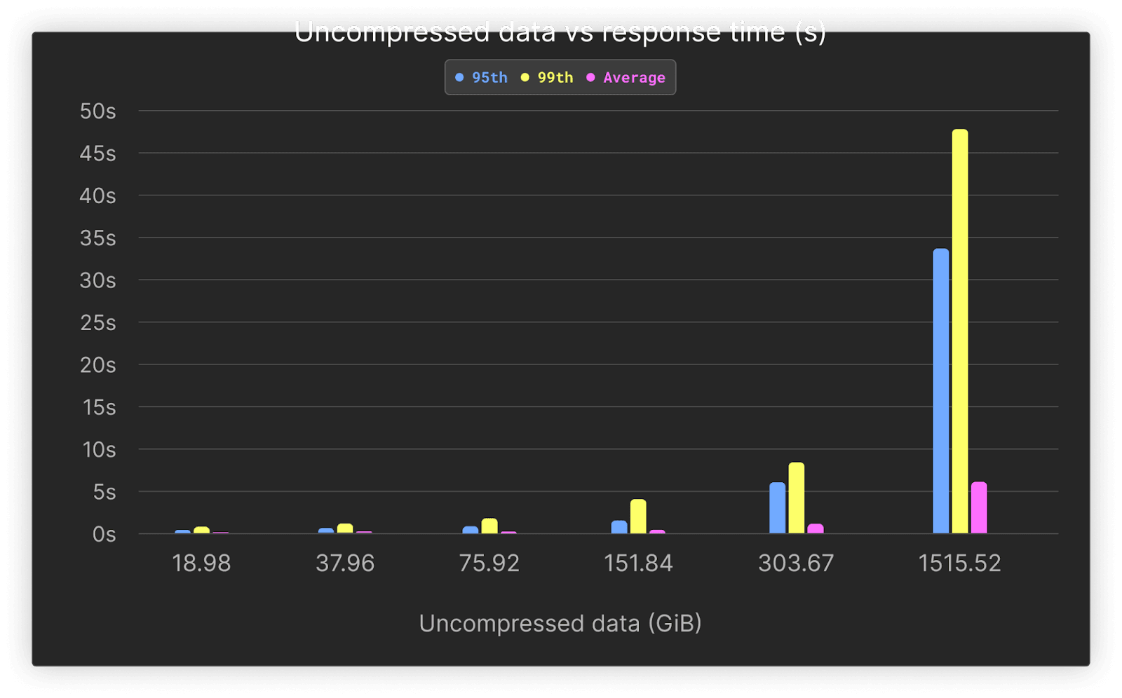
Average performance remains under 1 second across all queries, up to 1 billion rows. As shown, query performance on most queries does not grade significantly as volumes grow, with better than linear performance thanks to ClickHouse’s sparse index.
Higher percentiles can be attributed to cold queries, with no warm-up time for our benchmark. As shown below, these slower queries are also associated with our final drill-down behavior, where we visualize the data over 30 days. This type of access is generally infrequent, with SREs focusing on narrower time frames. Despite this, average performance remains below 6s even for our largest test at 1.5TiB.
Below, we show the average performance of our dashboard visualizations for different drill-downs and data volumes.
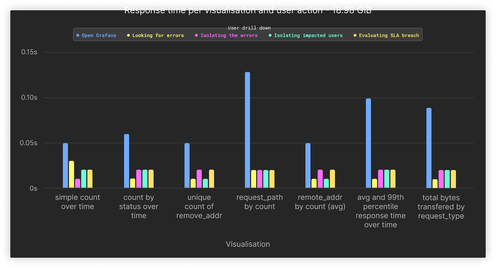
At 66 million rows or 19GiB, performance for all queries averages under 0.1s.
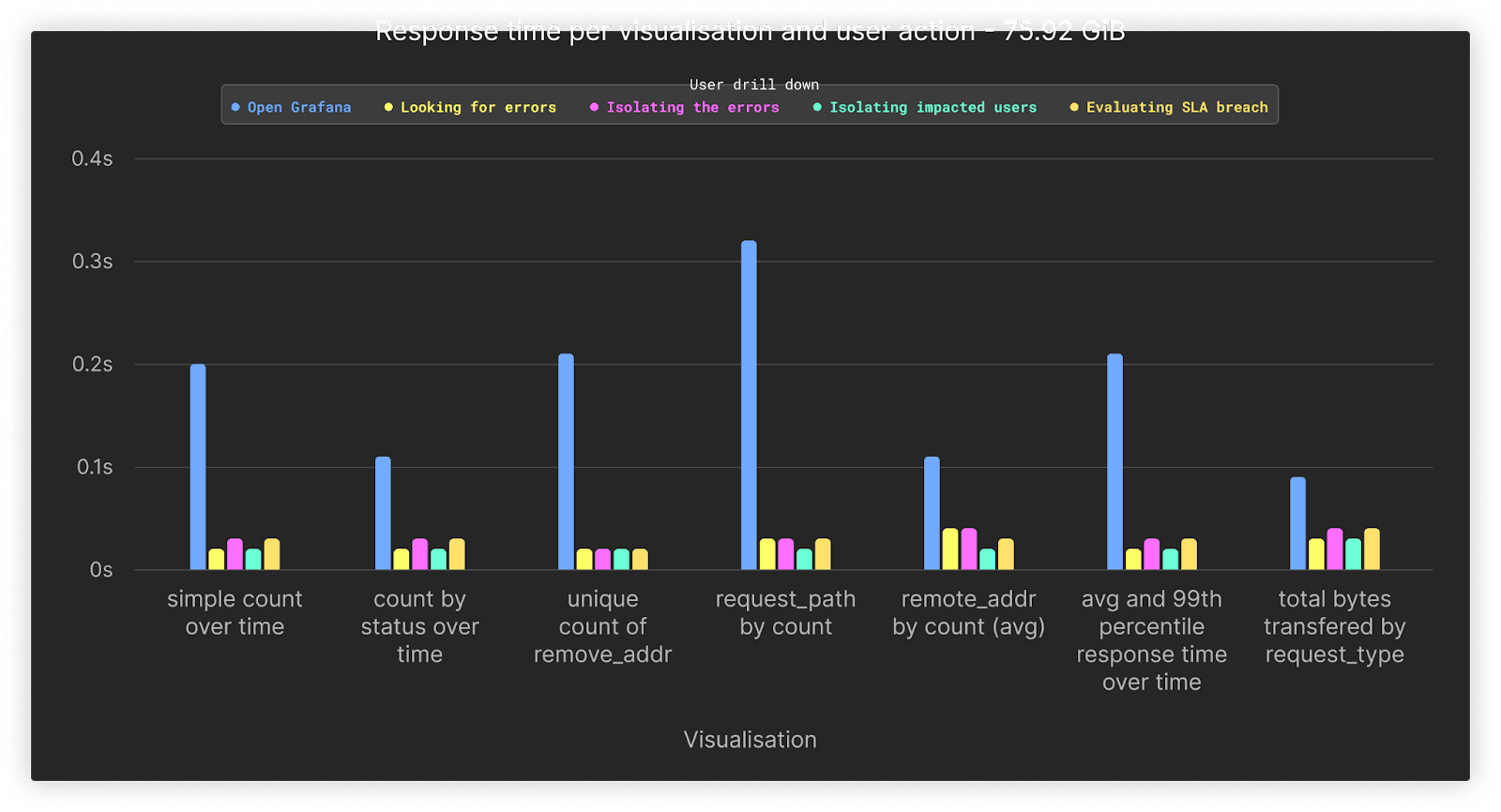
Increasing the data over our previous test by x4 shows the performance for 267 million rows or 76GiB. All queries remain comparable in performance to the previous test despite the increase in data.
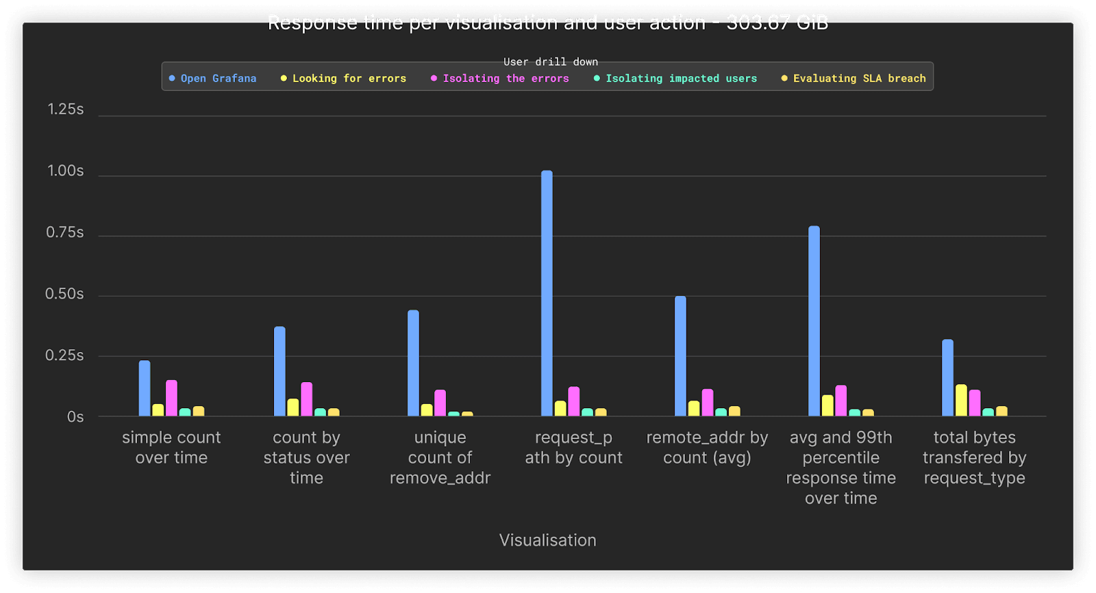
Performance of all queries remains, on average, under 1s if we increase our data volumes by a further factor of 4 to 300GiB or approximately 1 billion rows.
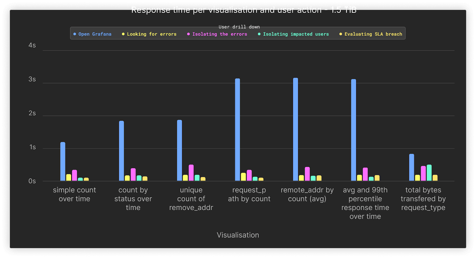
For our final test, we increased the volume to 1.5TiB of uncompressed data or 5.3 billion rows. Our queries associated with the first opening of the dashboard, during which no filters other than time are applied, represent the slowest queries at around 1.5 to 3s. All queries that involve drill-downs are completed comfortably under a second.
An astute reader will notice that we don’t include the performance of our final set of queries above, associated with when the user “zooms out” to cover the entire month. These represent the most expensive queries, with their timing distorting the above charts. We therefore present these separately below.
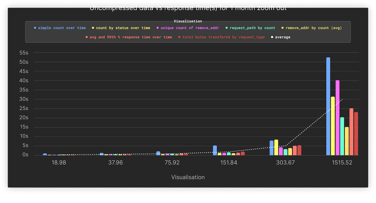
As shown, the performance of this action heavily depends on the volume of data being queried, with performance remaining on average under 5s until the larger 1.5TiB load. We expect these queries, which cover the full dataset, to be infrequent and not typical of the usual SRE workflow. However, even if these queries are rare, we can take measures to improve their performance using Clickhouse features. We explore these in the context of this larger dataset below.
Improving query performance
The above results show the performance of most of our dashboard queries to be, on average, below a few seconds. Our “zoom-out” query, where our SRE attempts to identify trends over a full month, takes up to 50 seconds. While this is not a complete linear scan, as we are still applying filters, this particular query is CPU-bound, with each of the two nodes in our Development service having only two cores. By default, queries are only executed on the receiving node for the query. These queries will, therefore, benefit from distributing computation across all nodes in the cluster, allowing four cores to be assigned to the aggregation.
In ClickHouse Cloud, this can be achieved by using parallel replicas. This feature allows the work for an aggregation query to be spread across all nodes in the cluster, reading from the same single shard. This feature, while experimental, is already in use for some workloads in ClickHouse Cloud and is expected to be generally available soon.
Below, we show the results when parallel replicas are enabled to use the full cluster resources for all queries issued as part of the final zoom-out step. The results here are for the largest dataset of 1.5TiB. Full results can be found here.
| simple count over time | count by status over time | unique count of remote_addr | request_path by count | remote_addr by count | average and 99th percentile response time transferred over time | total bytes transferred by request_type | |
|---|---|---|---|---|---|---|---|
| With Parallel Replicas | 24.8 | 10.81 | 10.84 | 9.74 | 9.75 | 9.31 | 8.89 |
| No Parallel Replicas | 52.46 | 31.35 | 40.26 | 20.41 | 15.14 | 25.29 | 23.2 |
| Speedup | 2.12 | 2.9 | 3.71 | 2.1 | 1.55 | 2.72 | 2.61 |
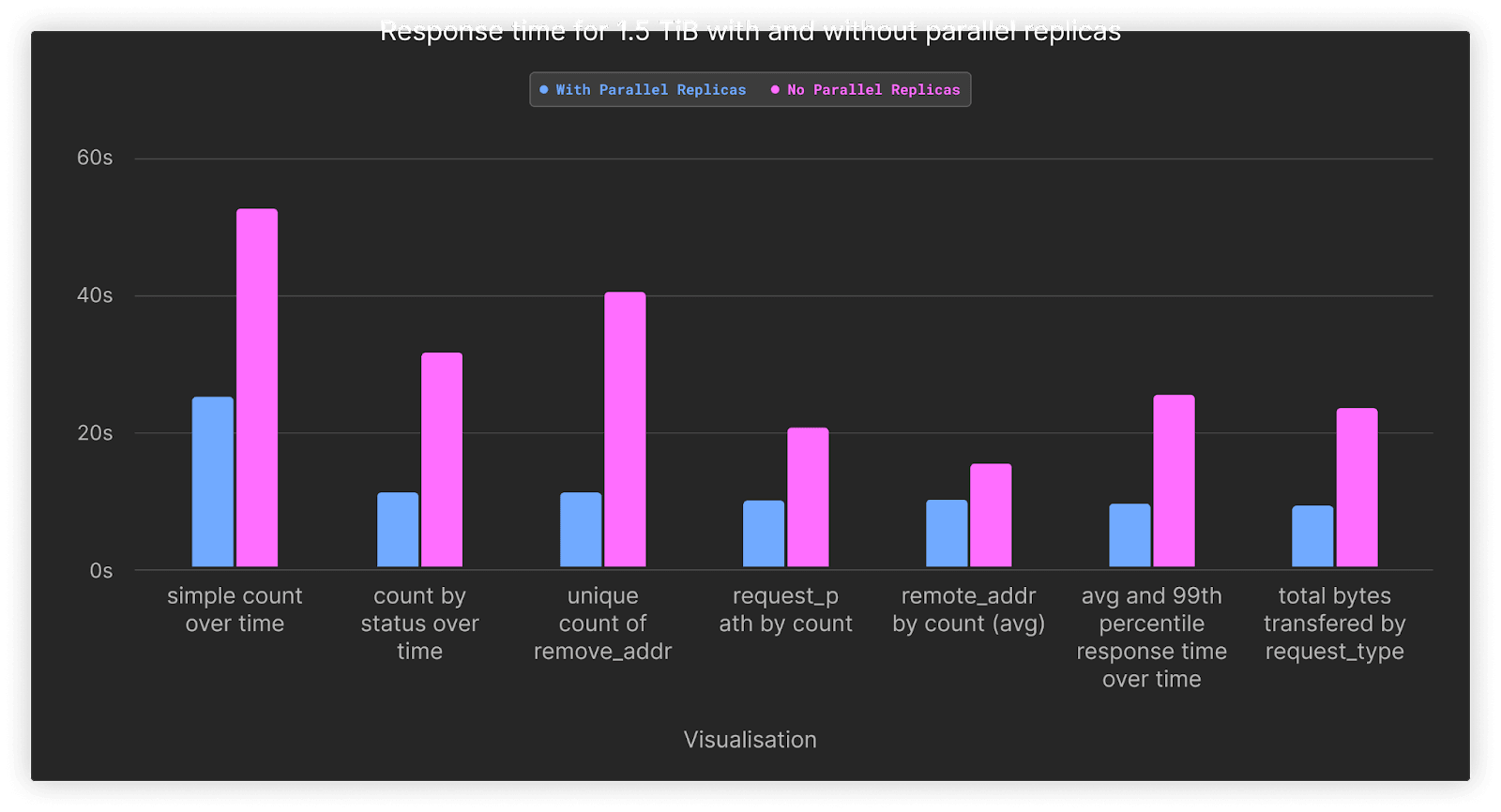
As shown, enabling parallel replicas speeds up our queries by, on average, 2.5x. This ensures our queries respond in at most 24s, with most completing in 10s. Note that based on our testing, parallel replicas only provide a benefit once a large number of rows needs to be aggregated. The cost of distribution exceeds the benefits for other smaller datasets. In future releases of ClickHouse, we plan to make the use of this feature more automatic vs. relying on the user to apply the appropriate settings manually based on data volume.
Cost analysis
ClickHouse
The cost of utilizing the Development tier of ClickHouse Cloud is mostly dominated by the compute units, with an additional charge for the data stored. In relative terms, the storage cost for this workload is minimal, thanks to the usage of object storage in ClickHouse cloud. Users are, therefore, encouraged to retain data for longer periods of time without the concern of accumulating cost.
- $0.2160 per hour. Assuming our service is always active this is approximately $0.2160 x 24 x 30 = $155.52
- $35.33 per TiB per month for compressed data
Based on this we can use a simple calculation to estimate our costs for the earlier volumes.
| Uncompressed size (GiB) | Compressed size (GiB) | Number of rows (millions) | Retain cost (1 month) for compute ($) | Storage cost ($) | Total Cost per month ($) |
|---|---|---|---|---|---|
| 18.98 | 1.37 | 66.75 | 155.52 | 0.05 | 155.57 |
| 37.96 | 2.96 | 133.49 | 155.52 | 0.1 | 155.62 |
| 75.92 | 5.42 | 267 | 155.52 | 0.19 | 155.71 |
| 151.84 | 10.68 | 534 | 155.52 | 0.37 | 155.89 |
| 303.67 | 20.73 | 1070 | 155.52 | 0.72 | 156.24 |
| 1515.52 | 93.24 | 5370 | 155.52 | 3.22 | $158.74 |
| 14336 | 1024 | 58976 | 155.52 | 35.33 | $190.85 |
As mentioned earlier, uncompressed size here can be considered equivalent to raw log formats in CSV and non-structured formats. It is clear our storage cost here is minimal, consuming $3 for our largest test case with 1.5TiB of uncompressed data.
Our final line in the above table would project the cost if we utilized the full 1TiB of compressed storage available with a Development tier. This could be achieved through either longer retainment of the data or greater volumes per month, which is equivalent to over 58b rows of data and 14TiB of uncompressed logs. This still only costs $190 per month. Due to the low cost of object storage, this is only $32 more than storing our largest 1.5TiB uncompressed test case!
WarpStream
The pricing exercise for WarpStream is simpler, with no complex queries to run. In this scenario, WarpStream acts as a cost-efficient and scalable buffer. We assume a significantly lower compression ratio of 4x over the wire since the data is not organized in a columnar fashion, and clients may be producing or consuming small batches, depending on their configuration. Finally, we’ll also assume 48 hours of retention is sufficient since WarpStream is just acting as a temporary buffer in front of ClickHouse and not the final destination. The costs for the full 14TiB are presented below.
| Uncompressed Size (GiB) | Throughput MiB/s | Compute cost for agent($) | Storage cost (2 days) ($) | S3 API Costs | Total Cost per month ($) |
|---|---|---|---|---|---|
| 18.98 | 1.8Kib/s | $21.4 | $0.007 | $58 | $80 |
| 37.96 | 3.6KiB/s | $21.4 | $0.014 | $58 | $80 |
| 75.92 | 7KiB/s | $21.4 | $0.028 | $58 | $80 |
| 151.84 | 14KiB/s | $21.4 | $0.057 | $58 | $80 |
| 303.67 | 29KiB/s | $21.4 | $0.116 | $58 | $80 |
| 1515.52 | 146KiB/s | $21.4 | $0.58 | $58 | $80 |
| 14336 | 1.38 MiB/s | $21.4 | $5.49 | $58 | $85 |
Above uses a Fly.io 2x shared-cpu-1x with 2GiB of RAM
Note that the WarpStream compute and S3 API costs are relatively “fixed” costs, with the workload size able to grow a further 5-10x without either of those costs increasing. This is because we need to run at least two Agents for high availability. However, even the two small Agents in this setup can easily tolerate a write volume of 10-20MiB/s, more than one order of magnitude than the highest row. The compute costs thus remain fixed.
In addition, the S3 API costs are also mostly fixed since the Agents have to generate one file every 250 ms irrespective of the load. However, as the write volume increases, so does batching, and the cost remains fixed until the total write throughput of the workload exceeds the maximum ingestion file size of 8MiB.
Summary
Below we present the total costs per month for a CGW stack for various log volumes.
| Uncompressed size (GiB) | WarpStream cost per month ($) | ClickHouse cost per month ($) | Total cost ($) |
|---|---|---|---|
| 18.98 | 80 | 155.57 | 235.57 |
| 37.96 | 80 | 155.62 | 235.62 |
| 75.92 | 80 | 155.71 | 235.71 |
| 151.84 | 80 | 155.89 | 235.89 |
| 303.67 | 80 | 156.24 | 236.89 |
| 1515.52 | 80 | 158.74 | 238.74 |
| 14336 | 85.43 | 190.85 | 276.28 |
The above does not include the cost for the OTEL collectors (or equivalent), which we assume will be run on the edge and represent a negligible overhead.
Cost comparisons
To give some relative comparison elements, we decided to compare the costs of our CGW stack against two leading solutions in the logging space, namely Datadog and Elastic Cloud.
The reader should remember that we are not performing an exact apples-to-apples comparison here as both Elastic and Datadog provide a comprehensive logging user experience beyond the main storage/querying feature. On the other hand, both alternative solutions presented do not include a Kafka or Kafka-compatible queuing mechanism.
However, from a functional standpoint, the main objective is the same, and the CGW is a valid alternative for the core logging use case. We display the cost differences in the table below, based on the data from the publicly available pricing calculators and the following hypotheses:
- The CGW Cost Per Month: Consists of the Warpstream + ClickHouse Cloud costs mentioned above and assumes using a Grafana Cloud free-tier instance.
- The Elastic Cloud Cost Per Month: Assumes an Elastic standard tier (minimum) running on a general-purpose hardware profile with 2 availability zones and 1 free Kibana instance. We also assume a 1 to 1 data compression ratio.
- The Datadog Cost Per Month: Assumes a 30-day-only retention period with a yearly commitment (30 days is the highest period with public pricing listed on datadoghq.com/pricing)
- Moreover, both alternative solutions presented do not include a Kafka or Kafka-compatible queuing mechanism that will have to be deployed and evaluated separately. We discarded this cost for alternative solutions.
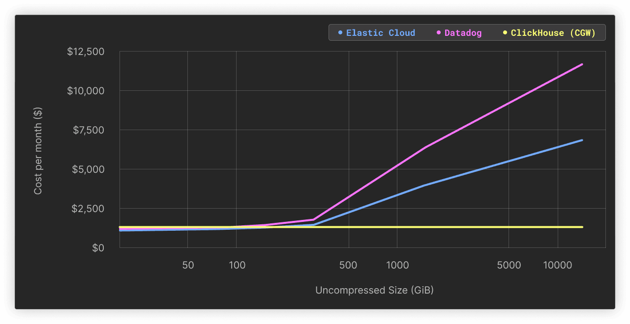
| Uncompressed size (GiB) | Compressed size (GiB) | Number of rows (millions) | CGW Cost Per Month ($) | Elastic Cloud Cost Per Month ($) | Elastic Cloud / CGW multiple | Datadog Cost Per Month ($) | Datadog / CGW multiple |
|---|---|---|---|---|---|---|---|
| 18.98 | 1.37 | 66.75 | 241 | $82 | x 0.3 | $143 | x 0.6 |
| 37.96 | 2.96 | 133.49 | 241.05 | $82 | x 0.3 | $143 | x 0.6 |
| 75.92 | 5.42 | 267 | 241.14 | $131 | x 0.5 | $234 | x 1.0 |
| 151.84 | 10.68 | 534 | 241.32 | $230 | x 1.0 | $415 | x 1.7 |
| 303.67 | 20.73 | 1070 | 241.67 | $428 | x 1.8 | $776 | x 3.2 |
| 1515.52 | 93.24 | 5370 | 244.17 | $3,193 | x 13.1 | $5,841 | x 23.9 |
| 14336 | 1024 | 58976 | 276.28 | $6,355 | x 23.0 | $11,628 | x 42.1 |
As displayed above, for any small workload (<150 GiB of uncompressed data), the almost static cost of the CGW stack is not really justified, and the alternative solutions are attractive. However, past this threshold, we quickly observe that the cost grows at a higher pace than the data volume managed for the alternative solutions, reaching multiples at x23 for Elastic Cloud and x42 for Datadog for 1.5 TiB worth of logs data.
Based on the results above, we conclude that the CGW stack presents a cost-effective alternative that can easily scale to a multi-terabyte scale without hurting the costs. This predictability of the cost presents a clear advantage to users who expect growth in their systems and want to avoid surprises in the future. Beyond this scale, the user can always decide to upgrade to a production-level ClickHouse Cloud service to keep up with ever-growing volumes. We expect the cost savings in this case, as volumes exceed 100TiB and even PiB, to be even more substantial, as evidenced by large CDN providers using ClickHouse for logs.
In addition to the cost efficiency, having access to a fully-fledged modern analytics store means that you can extend the use case beyond basic log storage and retrieval, benefiting from ClickHouse’s vibrant integrations ecosystem. One example is that you can decide to store large volumes of logs in Parquet format in a remote object bucket for archival purposes using the S3 table function, expanding your retention capabilities.
Conclusion
In this post, we’ve presented the CGW stack, a logging solution based on ClickHouse Cloud, WarpStream, and Grafana. If using a ClickHouse Cloud Development service, this stack provides an efficient means of storing up to 14TiB of uncompressed data per month for less than $300. This is 23x more cost-efficient than the comparable Elastic Cloud deployment and up to 42x less expensive than DataDog for the same volume of data.