Welcome to our first release post of 2024, although it’s actually for a release that sneaked in at the end of 2023! ClickHouse version 23.12 contains 21 new features, 18 performance optimisations, and 37 bug fixes.
We’re going to cover a small subset of the new features in this blog post, but the release also covers the ability to ORDER BY ALL, generate a Short Unique Identifiers (SQID) From Numbers, find the frequency of a signal using a new Fourier transform-based seriesPeriodDetectFFT function, support for SHA-512/256, indices on ALIAS columns, clean deleted records after a lightweight delete operation via APPLY DELETED MASK, lower memory usage for hash joins and faster counting for Merge tables.
In terms of integrations, we also have improvements for ClickHouse’s PowerBI, Metabase, dbt, Apache Beam and Kafka connectors.
New Contributors
As always, we send a special welcome to all the new contributors in 23.12! ClickHouse's popularity is, in large part, due to the efforts of the community that contributes. Seeing that community grow is always humbling.
Below are the names of the new contributors:
Andrei Fedotov, Chen Lixiang, Gagan Goel, James Nock, Natalya Chizhonkova, Ryan Jacobs, Sergey Suvorov, Shani Elharrar, Zhuo Qiu, andrewzolotukhin, hdhoang, and skyoct.
If you see your name here, please reach out to us...but we will be finding you on twitter, etc as well.
You can also view the slides from the presentation.
Refreshable Materialized Views
Contributed by Michael Kolupaev, Michael Guzov
Users new to ClickHouse often find themselves exploring materialized views to solve a wide range of data and query problems, from accelerating aggregation queries to data transformation tasks at insert time. At this point, the same users also often encounter a common source of confusion - the expectation that Materialized Views in ClickHouse are similar to those they have used in other databases when they are just a query trigger executed at insert time on newly inserted rows! More precisely, when rows are inserted into ClickHouse as a block (usually consisting of at least 1000 rows), the query defined for a Materialized View is executed on the block, with the results stored in a different target table. This process is described succinctly in a recent video by our colleague Mark:
This feature is extremely powerful and, like most things in ClickHouse, has been deliberately designed for scale, with views updated incrementally as new data is inserted. However, there are use cases where this incremental process is not required or is not applicable. Some problems are either incompatible with an incremental approach or don't require real-time updates, with a periodic rebuild being more appropriate. For example, you may want to periodically perform a complete recomputation of a view over the full dataset because it uses a complex join, which is incompatible with an incremental approach.
In 23.12, we are pleased to announce the addition of Refreshable Materialized Views as an experimental feature to address these use cases! As well as allowing views to consist of a query that is periodically executed, with the results set to a target table, this feature can also be used to perform cron tasks in ClickHouse, e.g., periodically export from or to external data sources.
This significant feature deserves its own blog post (stay tuned!), especially given the number of problems it can potentially solve.
As an example, to introduce the syntax, let's consider a problem that may be challenging to address with a traditional incremental materialized view or even a classic view.
Consider the example we use for our integration with dbt. This consists of a small IMDB dataset with the following relational schema. This dataset originates from the relational dataset repository.
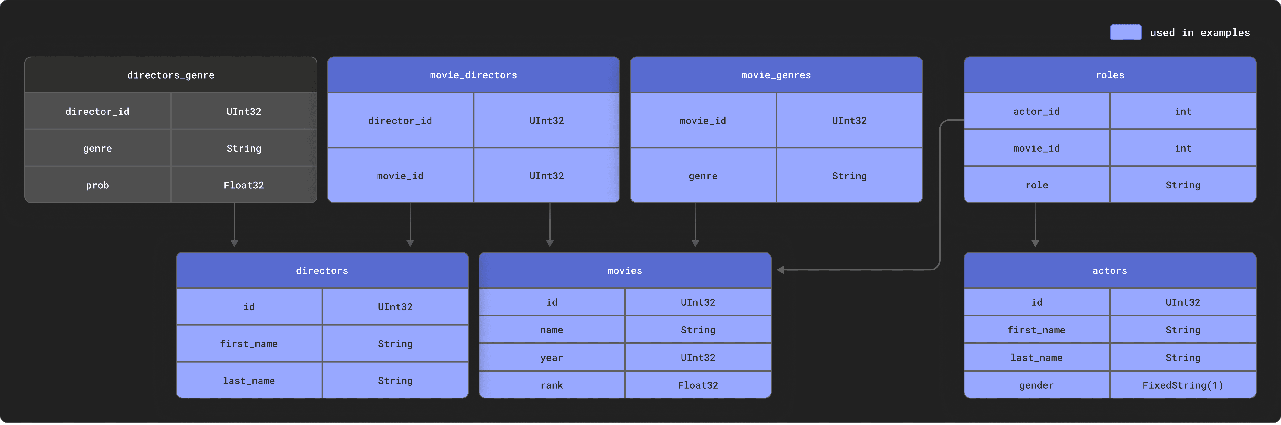
Assuming you’ve created and populated these tables in ClickHouse, as described in our documentation, the following query can be used to compute a summary of each actor, ordered by the most movie appearances.
SELECT
	id,
	any(actor_name) AS name,
	uniqExact(movie_id) AS num_movies,
	avg(rank) AS avg_rank,
	uniqExact(genre) AS unique_genres,
	uniqExact(director_name) AS uniq_directors,
	max(created_at) AS updated_at
FROM
(
	SELECT
    	imdb.actors.id AS id,
    	concat(imdb.actors.first_name, ' ', imdb.actors.last_name) AS actor_name,
    	imdb.movies.id AS movie_id,
    	imdb.movies.rank AS rank,
    	genre,
    	concat(imdb.directors.first_name, ' ', imdb.directors.last_name) AS director_name,
    	created_at
	FROM imdb.actors
	INNER JOIN imdb.roles ON imdb.roles.actor_id = imdb.actors.id
	LEFT JOIN imdb.movies ON imdb.movies.id = imdb.roles.movie_id
	LEFT JOIN imdb.genres ON imdb.genres.movie_id = imdb.movies.id
	LEFT JOIN imdb.movie_directors ON imdb.movie_directors.movie_id = imdb.movies.id
	LEFT JOIN imdb.directors ON imdb.directors.id = imdb.movie_directors.director_id
)
GROUP BY id
ORDER BY num_movies DESC
LIMIT 5

┌─────id─┬─name─────────┬─num_movies─┬───────────avg_rank─┬─unique_genres─┬─uniq_directors─┬──────────updated_at─┐
│  45332 │ Mel Blanc    │   	 909 │ 5.7884792542982515 │   		   19 │   		 148   │ 2024-01-08 15:44:31 │
│ 621468 │ Bess Flowers │   	 672 │  5.540605094212635 │   		   20 │   		 301   │ 2024-01-08 15:44:31 │
│ 283127 │ Tom London   │   	 549 │ 2.8057034230202023 │   		   18 │   		 208   │ 2024-01-08 15:44:31 │
│  41669 │ Adoor Bhasi  │   	 544 │         		    0 │     	    4 │   		 121   │ 2024-01-08 15:44:31 │
│  89951 │ Edmund Cobb  │   	 544 │   2.72430730046193 │   		   17 │   		 203   │ 2024-01-08 15:44:31 │
└────────┴──────────────┴────────────┴────────────────────┴───────────────┴────────────────┴─────────────────────┘

5 rows in set. Elapsed: 1.207 sec. Processed 5.49 million rows, 88.27 MB (4.55 million rows/s., 73.10 MB/s.)
Peak memory usage: 1.44 GiB.
Admittedly, this isn't the slowest query, but let's assume a user needs this to be a lot faster and computationally cheaper for an application. Suppose that this dataset is also subject to constant updates - movies are constantly released with new actors and directors also emerging.
A normal view here isn't going to help, and converting this to an incremental materialized view would be challenging: only changes to the table on the left side of a join will be reflected, requiring multiple chained views and significant complexity.
With 23.12, we can create a Refreshable Materialized View that will periodically run the above query and atomically replace the results in a target table. While this won't be as real-time in its updates as an incremental view, it will likely be sufficient for a dataset that is unlikely to be updated as frequently.
Let's first create our target table for the results:
CREATE TABLE imdb.actor_summary
(
	`id` UInt32,
	`name` String,
	`num_movies` UInt16,
	`avg_rank` Float32,
	`unique_genres` UInt16,
	`uniq_directors` UInt16,
	`updated_at` DateTime
)
ENGINE = MergeTree
ORDER BY num_movies
Creating the Refreshable Materialized View uses the same syntax as an incremental, except we introduce a REFRESH clause specifying the period on which the query should be executed. Note that we removed the limit for the query to store the full results. This view type imposes no restrictions on the SELECT clause.
//enable experimental feature
SET allow_experimental_refreshable_materialized_view = 1

CREATE MATERIALIZED VIEW imdb.actor_summary_mv
REFRESH EVERY 1 MINUTE TO imdb.actor_summary AS
SELECT
	id,
	any(actor_name) AS name,
	uniqExact(movie_id) AS num_movies,
	avg(rank) AS avg_rank,
	uniqExact(genre) AS unique_genres,
	uniqExact(director_name) AS uniq_directors,
	max(created_at) AS updated_at
FROM
(
	SELECT
    	imdb.actors.id AS id,
    	concat(imdb.actors.first_name, ' ', imdb.actors.last_name) AS actor_name,
    	imdb.movies.id AS movie_id,
    	imdb.movies.rank AS rank,
    	genre,
    	concat(imdb.directors.first_name, ' ', imdb.directors.last_name) AS director_name,
    	created_at
	FROM imdb.actors
	INNER JOIN imdb.roles ON imdb.roles.actor_id = imdb.actors.id
	LEFT JOIN imdb.movies ON imdb.movies.id = imdb.roles.movie_id
	LEFT JOIN imdb.genres ON imdb.genres.movie_id = imdb.movies.id
	LEFT JOIN imdb.movie_directors ON imdb.movie_directors.movie_id = imdb.movies.id
	LEFT JOIN imdb.directors ON imdb.directors.id = imdb.movie_directors.director_id
)
GROUP BY id
ORDER BY num_movies DESC
The view will execute immediately and every minute thereafter as configured to ensure updates to the source table are reflected. Our previous query to obtain a summary of actors becomes syntactically simpler and significantly faster!
SELECT *
FROM imdb.actor_summary
ORDER BY num_movies DESC
LIMIT 5

┌─────id─┬─name─────────┬─num_movies─┬──avg_rank─┬─unique_genres─┬─uniq_directors─┬──────────updated_at─┐
│  45332 │ Mel Blanc    │   	 909 │ 5.7884793 │   		 19  │   		 148  │ 2024-01-09 10:12:57 │
│ 621468 │ Bess Flowers │   	 672 │  5.540605 │   		 20  │   		 301  │ 2024-01-09 10:12:57 │
│ 283127 │ Tom London   │   	 549 │ 2.8057034 │   		 18  │   		 208  │ 2024-01-09 10:12:57 │
│ 356804 │ Bud Osborne  │   	 544 │ 1.9575342 │   		 16  │   		 157  │ 2024-01-09 10:12:57 │
│  41669 │ Adoor Bhasi  │   	 544 │		   0 │    		  4	 │   		 121  │ 2024-01-09 10:12:57 │
└────────┴──────────────┴────────────┴───────────┴───────────────┴────────────────┴─────────────────────┘

5 rows in set. Elapsed: 0.003 sec. Processed 6.71 thousand rows, 275.62 KB (2.30 million rows/s., 94.35 MB/s.)
Peak memory usage: 1.19 MiB.
Suppose we add a new actor, "Clicky McClickHouse" to our source data who happens to have appeared in a lot of films!
INSERT INTO imdb.actors VALUES (845466, 'Clicky', 'McClickHouse', 'M');
INSERT INTO imdb.roles SELECT
	845466 AS actor_id,
	id AS movie_id,
	'Himself' AS role,
	now() AS created_at
FROM imdb.movies
LIMIT 10000, 910

0 rows in set. Elapsed: 0.006 sec. Processed 10.91 thousand rows, 43.64 KB (1.84 million rows/s., 7.36 MB/s.)
Peak memory usage: 231.79 KiB.
Less than 60 seconds later, our target table is updated to reflect the prolific nature of Clicky’s acting:
SELECT *
FROM imdb.actor_summary
ORDER BY num_movies DESC
LIMIT 5

┌─────id─┬─name────────────────┬─num_movies─┬──avg_rank─┬unique_genres─┬─uniq_directors─┬──────────updated_at─┐
│ 845466 │ Clicky McClickHouse │    	910 │ 1.4687939 │        	21 │        	662 │ 2024-01-09 10:45:04 │
│  45332 │ Mel Blanc       	   │    	909 │ 5.7884793 │        	19 │        	148 │ 2024-01-09 10:12:57 │
│ 621468 │ Bess Flowers    	   │    	672 │  5.540605 │        	20 │        	301 │ 2024-01-09 10:12:57 │
│ 283127 │ Tom London      	   │    	549 │ 2.8057034 │        	18 │        	208 │ 2024-01-09 10:12:57 │
│ 356804 │ Bud Osborne     	   │    	544 │ 1.9575342 │        	16 │        	157 │ 2024-01-09 10:12:57 │
└────────┴─────────────────────┴────────────┴───────────┴──────────────┴────────────────┴─────────────────────┘

5 rows in set. Elapsed: 0.003 sec. Processed 6.71 thousand rows, 275.66 KB (2.20 million rows/s., 90.31 MB/s.)
Peak memory usage: 1.19 MiB.
This example represents a simple application of Refreshable Materialized Views. This feature has potentially much broader applications. The periodic nature of the query execution means it could potentially be used for periodic imports or exports to external data sources. Furthermore, these views can be chained with a DEPENDS clause to create dependencies between views, thereby allowing complex workflows to be constructed. For further details, see the CREATE VIEW documentation.
We’d love to know how you are utilizing this feature and the problems it allows you to solve more efficiently now!
Optimizations For FINAL
Contributed by Maksim Kita
Automatic incremental background data transformation is an important concept in ClickHouse, allowing high data ingestion rates to be sustained at scale while continuously applying table engine-specific data modifications when data parts are merged in the background. For example, the ReplacingMergeTree engine retains only the most recently inserted version of a row based on the row’s sorting key column values and the creation timestamp of its containing data part when parts are merged. The AggregatingMergeTree engine collapses rows with equal sorting key values into an aggregated row during part merges.
As long as more than one part exists for a table, the table data is only in an intermediate state, i.e. outdated rows may exist for ReplacingMergeTree tables, and not all rows may have been aggregated yet for AggregatingMergeTree tables. In scenarios with continuous data ingestion (e.g. real-time streaming scenarios), it is almost always the case that multiple parts exist for a table. Luckily, ClickHouse has you covered: ClickHouse provides FINAL as a modifier for the FROM clause of SELECT queries (e.g. SELECT ... FROM table FINAL), which applies missing data transformations on the fly at query time. While this is convenient and decouples the query result from the progress of background merges, FINAL may also slow down queries and increase memory consumption.
Before ClickHouse version 20.5, SELECTs with FINAL were executed in a single-threaded fashion: The selected data was read from the parts by a single thread in physical order (based on the table's sorting key) while being merged and transformed.
ClickHouse 20.5 introduced parallel processing of SELECTs with FINAL: All selected data is split into groups with a distinct sorting key range per group and processed (read, merged, and transformed) concurrently by multiple threads.
ClickHouse 23.12 goes one important step further and divides the table data matching the query’s WHERE clause into non-intersecting and intersecting ranges based on sorting key values. All non-intersecting data ranges are processed in parallel as if no FINAL modifier was used in the query. This leaves only the intersecting data ranges, for which the table engine’s merge logic is applied with the parallel processing approach introduced by ClickHouse 20.5.
Additionally, for a FINAL query, ClickHouse no longer tries to merge data across different partitions if the table’s partition key is a prefix of the table’s sorting key.
The following diagram sketches this new processing logic for SELECT queries with FINAL:
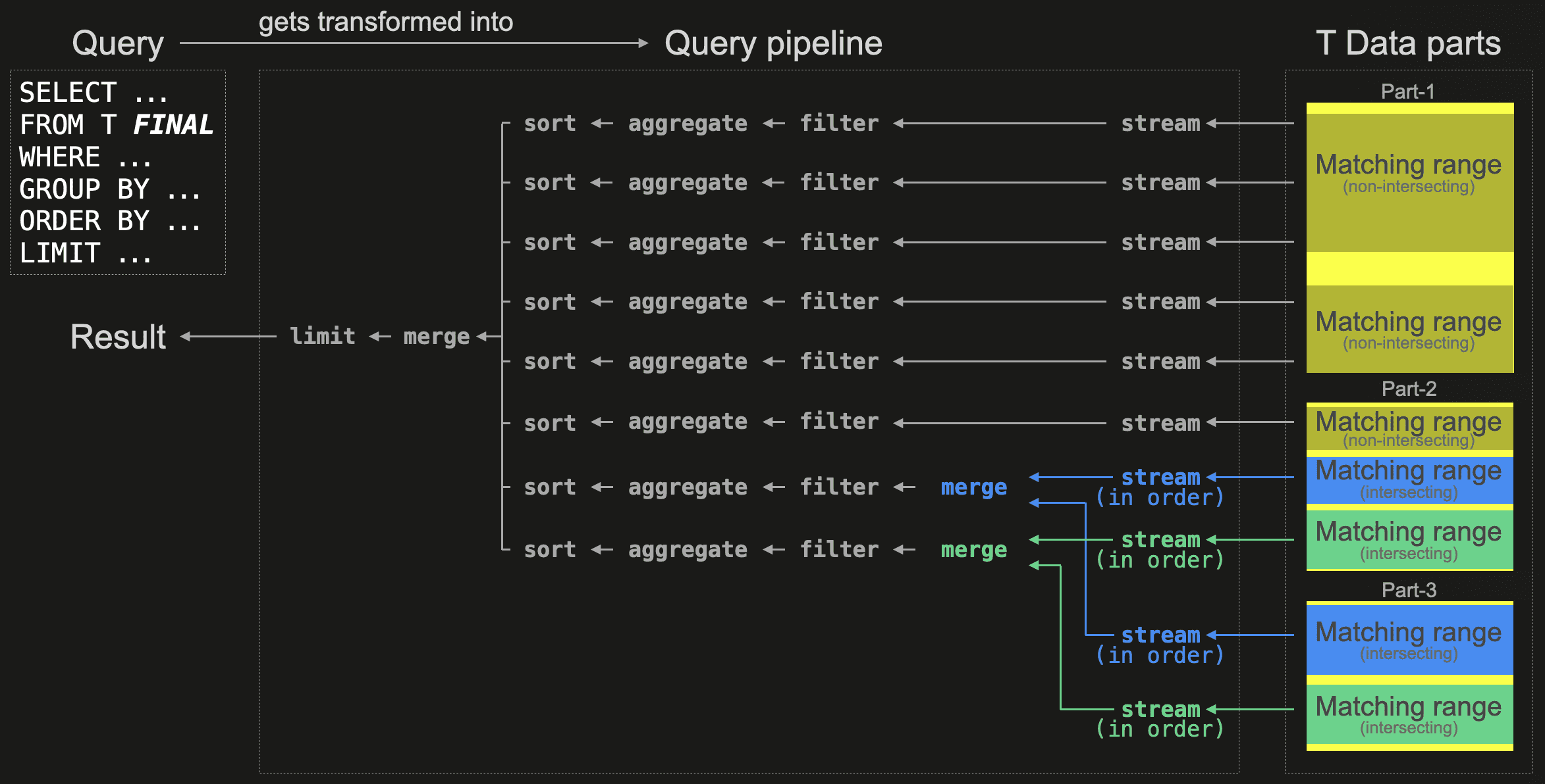
To parallelize data processing, the query gets transformed into a query pipeline - the query’s physical operator plan consisting of multiple independent execution lanes that concurrently stream, filter, aggregate, and sort disjoint ranges of the selected table data. The number of independent execution lanes depends on the max_threads setting, which by default is set to the number of available CPU cores. In our example above, the ClickHouse server running the query has 8 CPU cores.
Because the query uses the FINAL modifier, ClickHouse uses the primary indexes of the table’s data parts at planning time when creating the physical operator plan.
First, all data ranges within the parts matching the query’s WHERE clause are identified and split into non-intersecting and intersecting ranges based on the table’s sorting key. Non-intersecting ranges are data areas that exist only in a single part and need no transformation. Conversely, rows in intersecting ranges potentially exist (based on sorting key values) in multiple parts and require special handling. Furthermore, in our example above, the query planner could split the selected intersecting ranges into two groups (marked in blue and green in the diagram) with a distinct sorting key range per group. With the created query pipeline, all matching non-intersecting data ranges (marked in yellow in the diagram) are processed concurrently as usual (as if the query had no FINAL clause at all) by spreading their processing evenly among some of the available execution lanes. Data from the selected intersecting data ranges is - per group - streamed in order, and the table engine-specific merge logic is applied before the data is processed as usual.
Note that when the number of rows with the same sorting key column values is low, the query performance will be approximately the same as if no FINAL is used. We demonstrate this with a concrete example. For this, we slightly modify the table from the UK property prices sample dataset and assume that the table stores data about current property offers instead of previously sold properties. We are using a ReplacingMergeTree table engine, allowing us to update the prices and other features of offered properties by simply inserting a new row with the same sorting key values:
CREATE TABLE uk_property_offers
(
    postcode1 LowCardinality(String),
    postcode2 LowCardinality(String),
    street LowCardinality(String),
    addr1 String,
    addr2 String,
    price UInt32,
    …
)
ENGINE = ReplacingMergeTree
ORDER BY (postcode1, postcode2, street, addr1, addr2);
Next, we insert ~15 million rows into the table.
We run a typical analytics query without the FINAL modifier on ClickHouse version 23.11, selecting the three most expensive primary postcodes:
SELECT
    postcode1,
    formatReadableQuantity(avg(price))
FROM uk_property_offers
GROUP BY postcode1
ORDER BY avg(price) DESC
LIMIT 3

┌─postcode1─┬─formatReadableQuantity(avg(price))─┐
│ W1A       │ 163.58 million                     │
│ NG90      │ 68.59 million                      │
│ CF99      │ 47.00 million                      │
└───────────┴────────────────────────────────────┘

3 rows in set. Elapsed: 0.037 sec. Processed 15.52 million rows, 91.36 MB (418.58 million rows/s., 2.46 GB/s.)
Peak memory usage: 881.08 KiB.
We run the same query on ClickHouse version 23.11 with FINAL:
SELECT
    postcode1,
    formatReadableQuantity(avg(price))
FROM uk_property_offers FINAL
GROUP BY postcode1
ORDER BY avg(price) DESC
LIMIT 3;

┌─postcode1─┬─formatReadableQuantity(avg(price))─┐
│ W1A       │ 163.58 million                     │
│ NG90      │ 68.59 million                      │
│ CF99      │ 47.00 million                      │
└───────────┴────────────────────────────────────┘

3 rows in set. Elapsed: 0.299 sec. Processed 15.59 million rows, 506.68 MB (57.19 million rows/s., 1.86 GB/s.)
Peak memory usage: 120.81 MiB.
Note that the query with FINAL runs ~10 times slower and uses significantly more main memory.
We run the query with FINAL modifier on ClickHouse 23.12:
SELECT
    postcode1,
    formatReadableQuantity(avg(price))
FROM uk_property_offers FINAL
GROUP BY postcode1
ORDER BY avg(price) DESC
LIMIT 3;

┌─postcode1─┬─formatReadableQuantity(avg(price))─┐
│ W1A       │ 163.58 million                     │
│ NG90      │ 68.59 million                      │
│ CF99      │ 47.00 million                      │
└───────────┴────────────────────────────────────┘

3 rows in set. Elapsed: 0.036 sec. Processed 15.52 million rows, 91.36 MB (434.42 million rows/s., 2.56 GB/s.)
Peak memory usage: 1.62 MiB.
The query runtime and memory usage stay approximately the same for our example data on 23.12, regardless of whether the FINAL modifier is used or not! :)
Vectorization improvements
In 23.12 several common queries have been significantly improved thanks to increased vectorization using SIMD instructions.
Faster min/max
Contributed by Raúl Marín
The min and max functions have been made faster thanks to changes which allow these functions to be vectorized with SIMD instructions. These changes should improve query performance when it is CPU bound and not limited by I/O or memory bandwidth. While these cases might be rare, the improvement can be significant. Consider the following, rather artificial example, where we compute the maximum number from 1 billion integers. The following was executed on an Intel(R) Xeon(R) Platinum 8259CL CPU @ 2.50GHz, with support for Intel AVX instructions.
In 23.11:
SELECT max(number)
FROM
(
	SELECT *
	FROM system.numbers
	LIMIT 1000000000
)

┌─max(number)─┐
│   999999999 │
└─────────────┘

1 row in set. Elapsed: 1.102 sec. Processed 1.00 billion rows, 8.00 GB (907.50 million rows/s., 7.26 GB/s.)
Peak memory usage: 65.55 KiB.
And now for 23.12:
┌─max(number)─┐
│   999999999 │
└─────────────┘

1 row in set. Elapsed: 0.482 sec. Processed 1.00 billion rows, 8.00 GB (2.07 billion rows/s., 16.59 GB/s.)
Peak memory usage: 62.59 KiB.
For a more realistic example, consider the following NOAA weather dataset, containing over 1 billion rows. Below we compute the maximum temperature ever recorded.
In 23.11:
SELECT max(tempMax) / 10
FROM noaa

┌─divide(max(tempMax), 10)─┐
│                 	56.7 │
└──────────────────────────┘

1 row in set. Elapsed: 0.428 sec. Processed 1.08 billion rows, 3.96 GB (2.52 billion rows/s., 9.26 GB/s.)
Peak memory usage: 873.76 KiB.
While the improvement in 23.12 isn’t quite as substantial as our earlier artificial example, we still obtain a 25% speedup!
┌─divide(max(tempMax), 10)─┐
│                     56.7 │
└──────────────────────────┘

1 row in set. Elapsed: 0.347 sec. Processed 1.08 billion rows, 3.96 GB (3.11 billion rows/s., 11.42 GB/s.)
Peak memory usage: 847.91 KiB.
Faster aggregation
Contributed by Anton Popov
Aggregation has also gotten faster thanks to an optimization for the case of identical keys spanning a block. ClickHouse processes data block-wise. During aggregation processing, ClickHouse uses a hash table for either storing a new, or updating an existing aggregation value for the grouping key values of each row within a processed block of rows. The grouping key values are used to determine the aggregation values’ location within the hash table. When all rows in a processed block have the same unique grouping key, ClickHouse needs to determine the location for the aggregation values only once, followed by a batch of value updates at that location, which can be vectorized well.
Let’s give it a try on an Apple M2 Max to see how we do.
SELECT number DIV 100000 AS k,
       avg(number) AS avg,
       max(number) as max,
       min(number) as min
FROM numbers_mt(1000000000)
GROUP BY k
ORDER BY k
LIMIT 10;
In 23.11:
┌─k─┬──────avg─┬────max─┬────min─┐
│ 0 │  49999.5 │  99999 │      0 │
│ 1 │ 149999.5 │ 199999 │ 100000 │
│ 2 │ 249999.5 │ 299999 │ 200000 │
│ 3 │ 349999.5 │ 399999 │ 300000 │
│ 4 │ 449999.5 │ 499999 │ 400000 │
│ 5 │ 549999.5 │ 599999 │ 500000 │
│ 6 │ 649999.5 │ 699999 │ 600000 │
│ 7 │ 749999.5 │ 799999 │ 700000 │
│ 8 │ 849999.5 │ 899999 │ 800000 │
│ 9 │ 949999.5 │ 999999 │ 900000 │
└───┴──────────┴────────┴────────┘

10 rows in set. Elapsed: 1.050 sec. Processed 908.92 million rows, 7.27 GB (865.66 million rows/s., 6.93 GB/s.)
And in 23.12:
┌─k─┬──────avg─┬────max─┬────min─┐
│ 0 │  49999.5 │  99999 │      0 │
│ 1 │ 149999.5 │ 199999 │ 100000 │
│ 2 │ 249999.5 │ 299999 │ 200000 │
│ 3 │ 349999.5 │ 399999 │ 300000 │
│ 4 │ 449999.5 │ 499999 │ 400000 │
│ 5 │ 549999.5 │ 599999 │ 500000 │
│ 6 │ 649999.5 │ 699999 │ 600000 │
│ 7 │ 749999.5 │ 799999 │ 700000 │
│ 8 │ 849999.5 │ 899999 │ 800000 │
│ 9 │ 949999.5 │ 999999 │ 900000 │
└───┴──────────┴────────┴────────┘

10 rows in set. Elapsed: 0.649 sec. Processed 966.48 million rows, 7.73 GB (1.49 billion rows/s., 11.91 GB/s.)
PASTE JOIN
Contributed by Yarik Briukhovetskyi
The PASTE JOIN is useful for joining multiple datasets where equivalent rows in each dataset refer to the same item. i.e. row n in the first dataset should join with row n in the second. We can then join the datasets by row number rather than specifying a joining key.
Let’s give it a try using the Quora Question Pairs2 dataset from the GLUE benchmark on Hugging Face. We split the training Parquet file into two:
questions.parquet which contains question1, question2, and idx labels.parquet which contains label and idx
We can then join the columns back together using the PASTE JOIN.
INSERT INTO FUNCTION file('/tmp/qn_labels.parquet') SELECT *
FROM
(
    SELECT *
    FROM `questions.parquet`
    ORDER BY idx ASC
) AS qn
PASTE JOIN
(
    SELECT *
    FROM `labels.parquet`
    ORDER BY idx ASC
) AS lab

Ok.

0 rows in set. Elapsed: 0.221 sec. Processed 727.69 thousand rows, 34.89 MB (3.30 million rows/s., 158.15 MB/s.)
Peak memory usage: 140.47 MiB.