We are super excited to share a trove of amazing features in 23.11
Release Summary
25 new features. 24 performance optimisations. 70 bug fixes.
A small subset of highlighted features are below…But the release covers the ability to concat with arbitrary types, a fileCluster function, keeper improvements, asynchronous loading of tables, an index on system.numbers, concurrency control mechanisms, aggressive retries of requests on S3 and a smaller than ever binary size! and so…much…more.
Join us on the upcoming December Community Call on 28 December if you want a preview into a few special “gifts” coming in this month.
New Contributors
As always, we send a special welcome to all the new contributors in 23.11! ClickHouse's popularity is, in large part, due to the efforts of the community that contributes. Seeing that community grow is always humbling.
If you see your name here, please reach out to us...but we will be finding you on twitter, etc as well.
Andrej Hoos, Arvind Pj, Chuan-Zheng Lee, James Seymour, Kevin Mingtarja, Oleg V. Kozlyuk, Philip Hallstrom, Sergey Kviatkevich, Shri Bodas, abakhmetev, edef, joelynch, johnnymatthews, konruvikt, melvynator, pppeace, rondo_1895, ruslandoga, slu, takakawa, tomtana, xleoken, 袁焊忠
S3Queue is production-ready
Contributed by Sergei Katkovskiy & Kseniia Sumarokova
In release 23.8 we announced the experimental release of the S3Queue table engine to drastically simplify incremental loads from S3. This new table engine allows the streaming consumption of data from S3. As files are added to a bucket, ClickHouse will automatically process these files and insert them into a designated table. With this capability, users can set up simple incremental pipelines with no additional code.
We are pleased to announce that this feature has been significantly improved since its experimental release and is now production ready! To celebrate, our YouTube celebrity Mark has prepared a video:
Column Statistics for PREWHERE
Contributed by Han Fei
Column statistics are a new experimental feature that enables better query optimization in ClickHouse. With this feature, you can let ClickHouse create (and automatically update) statistics for columns in tables with a MergeTree-family engine. These statistics are stored inside the table’s parts in a small single statistics_(column_name).stat file, which is a generic container file for different types of statistics for every column that has statistics enabled. This ensures lightweight access to column statistics. As of today, the only type of column statistics supported are t-digests. Additional types are planned, though.
One first example where column statistics enable better optimizations is the column processing order in multi-stage PREWHERE filtering. We sketch this with a figure:
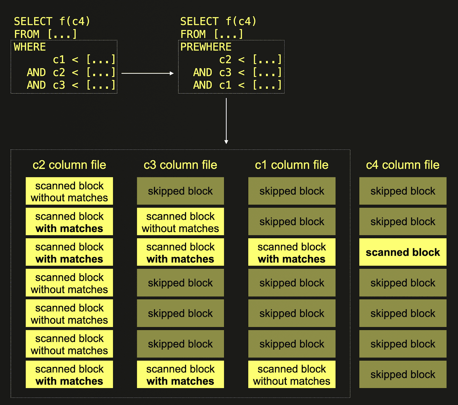
The query in the top left corner of the figure has a WHERE clause which consists of multiple AND-connected filter conditions. ClickHouse has an optimization that tries to evaluate the filters with the least possible amount of data scanned. This optimization is called multi-stage PREWHERE, and it is based on the idea that we can read the filter columns sequentially, i.e. column by column, and with every iteration, check only the blocks that contain at least one row that "survived" (= matched) the previous filter. The number of blocks to evaluate for each filter decreases monotonically.
Not surprisingly, this optimization works best when the filter that produces the smallest number of surviving blocks is evaluated first - in this case, ClickHouse needs to scan only a few blocks to evaluate the remaining filters. Of course, it is not possible to know how many blocks with matching rows survive each filter, so ClickHouse needs to make a guess to determine the optimal order in which the filters are executed. With column statistics, ClickHouse is able to estimate the number of matching rows / surviving blocks much more precisely, and therefore, multi-stage PREWHERE as an optimization becomes more effective.
In the example, ClickHouse utilizes column statistics to automatically determine that the filter condition on column c2 is the most selective one, i.e. it drops the most blocks. Therefore, processing starts with c2. All blocks from column c2 are scanned, and the filter predicate is evaluated for each row. Next, the filter evaluation is performed for column c3, but only on blocks with rows that had at least one match on the c2 filter in c2’s corresponding blocks. Because the filter condition on column c1 is the least selective one, the blocks of this column are processed last. Again, only those blocks are scanned (and the filter predicate is evaluated for each row), where the corresponding blocks from c2 and c3 both had predicate matches. From all other columns that need to be scanned and processed for the query run, ClickHouse only needs to scan those blocks from disk where all corresponding PREWHERE columns had predicate matches.
Let’s demonstrate this with a concrete example.
We create an example table and insert 10 million rows:
CREATE OR REPLACE TABLE example
(
    `a` Float64,
    `b` Int64,
    `c` Decimal64(4),
    `pk` String
)
ENGINE = MergeTree
ORDER BY pk;

INSERT INTO example SELECT
    number,
    number,
    number,
    generateUUIDv4()
FROM system.numbers
LIMIT 10_000_000
Next, we run a query with multiple AND-connected filter conditions in the WHERE clause. Note that we disable the PREWHERE optimization:
SELECT count()
FROM example
WHERE b < 10 AND a < 10 AND c < 10
SETTINGS optimize_move_to_prewhere = 0

┌─count()─┐
│      10 │
└─────────┘

1 row in set. Elapsed: 0.057 sec. Processed 10.00 million rows, 240.00 MB (176.00 million rows/s., 4.22 GB/s.)
Peak memory usage: 162.42 KiB.
We can see that the query processed 240 MB of column data.
Now we run the same query with (multi-stage) PREWHERE enabled:
SELECT count()
FROM example
WHERE b < 10 AND a < 10 AND c < 10

┌─count()─┐
│      10 │
└─────────┘

1 row in set. Elapsed: 0.032 sec. Processed 10.00 million rows, 160.42 MB (308.66 million rows/s., 4.95 GB/s.)
Peak memory usage: 171.74 KiB.
This time, the query processed 160 MB of column data.
Next, we enable the column statistics feature and enable and materialize t-digest-based statistics for three of our table’s columns
SET allow_experimental_statistic = 1;
ALTER TABLE example ADD STATISTIC a, b, c TYPE tdigest;
ALTER TABLE example MATERIALIZE STATISTIC a, b, c TYPE tdigest;
Running our example query with column statistic optimizations enabled:
SELECT count()
FROM example
WHERE b < 10 AND a < 10 AND c < 10
SETTINGS allow_statistic_optimize = 1

┌─count()─┐
│      10 │
└─────────┘

1 row in set. Elapsed: 0.012 sec. Processed 10.00 million rows, 80.85 MB (848.47 million rows/s., 6.86 GB/s.)
Peak memory usage: 160.25 KiB.
The query processed 80 MB of column data.
But this is just the beginning. Column statistics will also be used for other impactful optimizations like join reordering or for making the low cardinality data type an automatic decision.
Stay tuned!
Parallel window functions
Contributed by Dmitriy Novik
Anyone who has done serious data analysis with SQL will appreciate the value of Window functions. Window functions have been available in ClickHouse since 21.5. PostgreSQL's documentation does a great job of summarizing this SQL capability:
A window function performs a calculation across a set of table rows that are somehow related to the current row. This is comparable to the type of calculation that can be done with an aggregate function. But unlike regular aggregate functions, the use of a window function does not cause rows to become grouped into a single output row - the rows retain their separate identities. The window function is able to access more than just the current row of the query result.
While window functions can be applied to some pretty complex problems, most users will encounter them when needing to perform simple operations such as moving averages (which need to consider multiple rows) or cumulative sums. As these specific queries are often visualized in popular tools such as Grafana, we're always excited to announce when their performance is appreciably improved. In 23.11, ClickHouse takes a huge leap forward in its implementation of window functions by ensuring their execution can be parallelized.
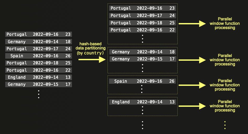
This parallelization is performed by exploiting the inherent bucketing capability of window functions: partitioning. When users specify that a window function should be partitioned by a column, a separate logical window is effectively created per partition i.e. if the column contains N distinct values, N windows need to be created. In 23.11, these partitions can effectively be constructed and evaluated in parallel.
As an example, consider the following query, which uses the NOAA weather dataset.
CREATE TABLE noaa
(
	`station_id` LowCardinality(String),
	`date` Date32,
	`tempAvg` Int32 COMMENT 'Average temperature (tenths of a degrees C)',
	`tempMax` Int32 COMMENT 'Maximum temperature (tenths of degrees C)',
	`tempMin` Int32 COMMENT 'Minimum temperature (tenths of degrees C)',
	`precipitation` UInt32 COMMENT 'Precipitation (tenths of mm)',
	`snowfall` UInt32 COMMENT 'Snowfall (mm)',
	`snowDepth` UInt32 COMMENT 'Snow depth (mm)',
	`percentDailySun` UInt8 COMMENT 'Daily percent of possible sunshine (percent)',
	`averageWindSpeed` UInt32 COMMENT 'Average daily wind speed (tenths of meters per second)',
	`maxWindSpeed` UInt32 COMMENT 'Peak gust wind speed (tenths of meters per second)',
	`weatherType` Enum8('Normal' = 0, 'Fog' = 1, 'Heavy Fog' = 2, 'Thunder' = 3, 'Small Hail' = 4, 'Hail' = 5, 'Glaze' = 6, 'Dust/Ash' = 7, 'Smoke/Haze' = 8, 'Blowing/Drifting Snow' = 9, 'Tornado' = 10, 'High Winds' = 11, 'Blowing Spray' = 12, 'Mist' = 13, 'Drizzle' = 14, 'Freezing Drizzle' = 15, 'Rain' = 16, 'Freezing Rain' = 17, 'Snow' = 18, 'Unknown Precipitation' = 19, 'Ground Fog' = 21, 'Freezing Fog' = 22),
	`location` Point,
	`elevation` Float32,
	`name` LowCardinality(String),
	`country` LowCardinality(String)
)
ENGINE = MergeTree
ORDER BY (country, date)


INSERT INTO noaa SELECT *
FROM s3('https://datasets-documentation.s3.eu-west-3.amazonaws.com/noaa/noaa_with_country.parquet')
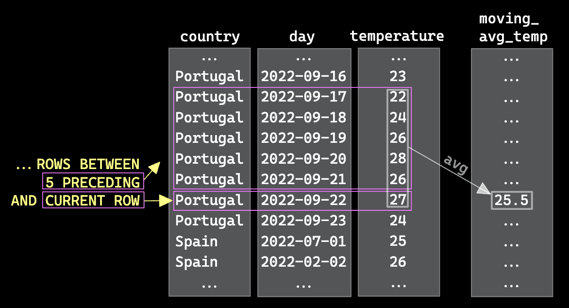
A simple window function might be used here to compute the moving average of temperature for every day and country. This requires us to partition by country (of which there are 214 in the dataset) and order by day. In computing the moving average we consider the last 5 datapoints.
SELECT
	country,
	day,
	max(tempAvg) AS temperature,
	avg(temperature) OVER (PARTITION BY country ORDER BY day ASC ROWS BETWEEN 5 PRECEDING AND CURRENT ROW) AS moving_avg_temp
FROM noaa
WHERE country != ''
GROUP BY
	country,
	date AS day
ORDER BY
	country ASC,
	day ASC
The intent of this simple function is best explained with a simple visualization.
Prior to 23.11, ClickHouse would have largely executed this function in parallel - with the notable exception of the window function. In cases where the query was not bound by other factors e.g. I/O, this could have potentially restricted performance.
In 23.10, on a 12 core machine with 96GiB of RAM, this query takes around 8.8s to run over the full 1 billion rows.
SELECT
	country,
	day,
	max(tempAvg) AS avg_temp,
	avg(avg_temp) OVER (PARTITION BY country ORDER BY day ASC ROWS BETWEEN 5 PRECEDING AND CURRENT ROW) AS moving_avg_temp
FROM noaa
WHERE country != ''
GROUP BY
	country,
	date AS day
ORDER BY
	country ASC,
	day ASC
LIMIT 10

┌─country─────┬────────day─┬─avg_temp─┬─────moving_avg_temp─┐
│ Afghanistan │ 1900-01-01 │  	-81   │             	-81 │
│ Afghanistan │ 1900-01-02 │ 	-145  │            	   -113 │
│ Afghanistan │ 1900-01-03 │ 	-139  │ -121.66666666666667 │
│ Afghanistan │ 1900-01-04 │ 	-107  │            	   -118 │
│ Afghanistan │ 1900-01-05 │  	-44   │          	 -103.2 │
│ Afghanistan │ 1900-01-06 │     0    │             	-86 │
│ Afghanistan │ 1900-01-07 │  	-71   │  -84.33333333333333 │
│ Afghanistan │ 1900-01-08 │  	-85   │  -74.33333333333333 │
│ Afghanistan │ 1900-01-09 │ 	-114  │  -70.16666666666667 │
│ Afghanistan │ 1900-01-10 │  	-71   │  -64.16666666666667 │
└─────────────┴────────────┴──────────┴─────────────────────┘

10 rows in set. Elapsed: 8.515 sec. Processed 1.05 billion rows, 7.02 GB (123.61 million rows/s., 824.61 MB/s.)
Peak memory usage: 1.13 GiB.
From 23.11, performance is improved by executing each partition parallel. Again, this is best described with a simple illustration.
Your actual gains here depend on a number of factors - not least having enough partitions and work per partition for the parallelization to provide a significant improvement. It also assumes the query is not bound by other factors. In our example below, we gain over a 10% improvement without needing to do anything!
SELECT
	country,
	day,
	max(tempAvg) AS avg_temp,
	avg(avg_temp) OVER (PARTITION BY country ORDER BY day ASC ROWS BETWEEN 5 PRECEDING AND CURRENT ROW) AS moving_avg_temp
FROM noaa
WHERE country != ''
GROUP BY
	country,
	date AS day
ORDER BY
	country ASC,
	day ASC
LIMIT 10

┌─country─────┬────────day─┬─avg_temp─┬─────moving_avg_temp─┐
│ Afghanistan │ 1900-01-01 │  	-81   │             	-81 │
│ Afghanistan │ 1900-01-02 │ 	-145  │            	   -113 │
│ Afghanistan │ 1900-01-03 │ 	-139  │ -121.66666666666667 │
│ Afghanistan │ 1900-01-04 │ 	-107  │            	   -118 │
│ Afghanistan │ 1900-01-05 │  	-44   │          	 -103.2 │
│ Afghanistan │ 1900-01-06 │     0    │             	-86 │
│ Afghanistan │ 1900-01-07 │  	-71   │  -84.33333333333333 │
│ Afghanistan │ 1900-01-08 │  	-85   │  -74.33333333333333 │
│ Afghanistan │ 1900-01-09 │ 	-114  │  -70.16666666666667 │
│ Afghanistan │ 1900-01-10 │  	-71   │  -64.16666666666667 │
└─────────────┴────────────┴──────────┴─────────────────────┘

10 rows in set. Elapsed: 7.571 sec. Processed 1.05 billion rows, 7.02 GB (139.03 million rows/s., 927.47 MB/s.)
Peak memory usage: 1.13 GiB.