We are super excited to share a trove of amazing features in 23.9
And, we already have a date for the 23.10 release, please register now to join the community call on November 2nd at 9:00 AM (PDT) / 6:00 PM (CET).
Release Summary
20 new features.
19 performance optimisations.
55 bug fixes.
A small subset of highlighted features are below…But the release covers dropping tables only if empty, auto-detection of JSON formats, support for long column names, improvements for converting numerics to datetimes, non-constant time zones, improved logging for backups, more MYSQL compatibility, the ability to generate temporary credentials, parallel reading of files for the INFILE clause, support for Tableau online and so…much…more.
New Contributors
As ever, we send a special welcome to all the new contributors in 23.9! ClickHouse's popularity is, in large part, due to the efforts of the community that contributes. Seeing that community grow is always humbling.
If you see your name here, please reach out to us...but we will be finding you on twitter, etc as well.
Alexander van Olst, Christian Clauss, CuiShuoGuo, Fern, George Gamezardashvili, Julia Kartseva, LaurieLY, Leonardo Maciel, Max Kainov, Petr Vasilev, Roman G, Tiakon, Tim Windelschmidt, Tomas Barton, Yinzheng-Sun, bakam412, priera, seshWCS, slvrtrn, wangtao.2077, xuzifu666, yur3k, Александр Нам.
Type Inference for JSON
Contributed by Pavel Kruglov
When will JSON be production-ready in ClickHouse?
Yes, we hear this a lot. A community call wouldn't be the same without this question! While we continue to work on this feature and have internally prioritized getting it to a production state at ClickHouse, we also believe that users often do not need all of the features and flexibility it will deliver. In the spirit of providing something that solves the majority of needs, we are pleased to introduce type inference for JSON.
This feature explicitly targets users who have well-structured JSON that is predictable. It allows a nested schema to be inferred from structured data, thus saving the user from having to manually define it. While this comes with some constraints, it accelerates the getting started experience.
For example, consider the following PyPI data. This data, which originates from BigQuery, where it is hosted as a public dataset, contains a row for every download of a Python package anywhere in the world (we've used it in earlier posts). As shown below, the schema here has multiple levels:
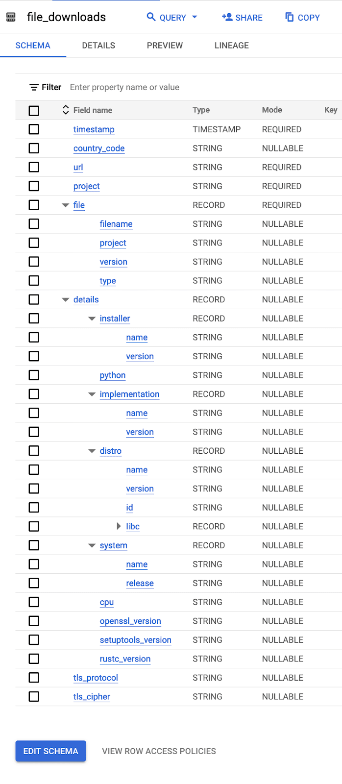
We've exported a sample of this data to a GCS bucket. Before 23.9, users of ClickHouse would need to define a schema in order to query this data. As shown below, this would prove quite tedious:
SELECT
	file.version,
	count() AS c
FROM s3('https://storage.googleapis.com/clickhouse_public_datasets/pypi/sample/*.json.gz', 'NOSIGN', 'JSONEachRow', 'timestamp DateTime64(9), country_code String, url String, project String, file Tuple(filename String, project String, type String, version String), details\tTuple(cpu String, distro Tuple(id String, libc Tuple(lib String, version String), name String, version String), implementation Tuple(name String, version String), installer Tuple(name String, version String), openssl_version String, python String, rustc_version String, setuptools_version String, system Tuple(name String, release String)), tls_protocol String, tls_cipher String')
WHERE project = 'requests'
GROUP BY file.version
ORDER BY c DESC
LIMIT 5

┌─file.version─┬──────c─┐
│ 2.31.0   	│ 268665 │
│ 2.27.1   	│  29931 │
│ 2.26.0   	│  11244 │
│ 2.25.1   	│  10081 │
│ 2.28.2   	│   8686 │
└──────────────┴────────┘

5 rows in set. Elapsed: 21.876 sec. Processed 26.42 million rows, 295.28 MB (1.21 million rows/s., 13.50 MB/s.)
Peak memory usage: 98.80 MiB.
Furthermore, it was impossible to create a table from a sample of this data and rely on schema inference. Instead, users would need to manually define the table schema before importing rows.
This overhead was acceptable for users who planned to retain the data and build a production service. For new users, or those wanting to perform ad hoc analysis, it represented a barrier to usage and added unnecessary friction. As of 23.9, the experience has been simplified and ClickHouse can infer the schema:
DESCRIBE TABLE s3('https://storage.googleapis.com/clickhouse_public_datasets/pypi/sample/*.json.gz')
FORMAT TSV

timestamp    Nullable(DateTime64(9))
country_code    Nullable(String)
url    Nullable(String)
project    Nullable(String)
file    Tuple(filename Nullable(String), project Nullable(String), type Nullable(String), version Nullable(String))
details    Tuple(cpu Nullable(String), distro Tuple(id Nullable(String), libc Tuple(lib Nullable(String), version Nullable(String)), name Nullable(String), version Nullable(String)), implementation Tuple(name Nullable(String), version Nullable(String)), installer Tuple(name Nullable(String), version Nullable(String)), openssl_version Nullable(String), python Nullable(String), rustc_version Nullable(String), setuptools_version Nullable(String), system Tuple(name Nullable(String), release Nullable(String)))
tls_protocol    Nullable(String)
tls_cipher    Nullable(String)

8 rows in set. Elapsed: 0.220 sec.
If we’re happy with the schema, we can then run the following query to find the most popular version of the requests library:
SELECT
	file.version,
	count() AS c
FROM s3('https://storage.googleapis.com/clickhouse_public_datasets/pypi/sample/*.json.gz')
WHERE project = 'requests'
GROUP BY file.version
ORDER BY c DESC
LIMIT 5

┌─file.version─┬──────c─┐
│ 2.31.0   	│ 268665 │
│ 2.27.1   	│  29931 │
│ 2.26.0   	│  11244 │
│ 2.25.1   	│  10081 │
│ 2.28.2   	│   8686 │
└──────────────┴────────┘

5 rows in set. Elapsed: 4.306 sec. Processed 26.46 million rows, 295.80 MB (6.14 million rows/s., 68.69 MB/s.)
Peak memory usage: 487.79 MiB.
This can also be used to define a table:
CREATE TABLE pypi
ENGINE = MergeTree
ORDER BY (project, timestamp) EMPTY AS
SELECT *
FROM s3('https://storage.googleapis.com/clickhouse_public_datasets/pypi/sample/*.json.gz') SETTINGS schema_inference_make_columns_nullable = 0

SHOW CREATE TABLE pypi FORMAT Vertical

CREATE TABLE default.pypi
(
	`timestamp` String,
	`country_code` String,
	`url` String,
	`project` String,
	`file` Tuple(filename String, project String, type String, version String),
	`details` Tuple(cpu String, distro Tuple(id String, libc Tuple(lib String, version String), name String, version String), implementation Tuple(name String, version String), installer Tuple(name String, version String), openssl_version String, python String, rustc_version String, setuptools_version String, system Tuple(name String, release String)),
	`tls_protocol` String,
	`tls_cipher` String
)
ENGINE = MergeTree
ORDER BY (project, timestamp)
SETTINGS index_granularity = 8192
Note how the structure is automatically inferred as nested Tuples. This schema inference does not produce an optimized schema. We recommend users still define the schema manually to optimize types and codecs for optimal performance, and use the inferred schema as a first pass or for ad-hoc analysis only.
So, how is this approach limited in comparison to the JSON type?
Firstly, the above requires all columns to be specified in the sample of data used for schema inference. By default, ClickHouse reads the first 25k rows or 32MB (whichever is less) in the data to establish these columns. During this inference step, the structure does not need to be consistent, and rows do not need to contain all columns. For example, imagine that we have the following messages:
{"a" : 1, "obj" : {"x" : 1}}
{"b" : 2, "obj" : {"y" : 2}}
If we ask ClickHouse to describe a potential table structure, it adds both a and b as potential columns.
DESCRIBE TABLE format(JSONEachRow, '{"a" : 1, "obj" : {"x" : 1}}, {"b" : 2, "obj" : {"y" : 2}}')
FORMAT TSV
a    Nullable(Int64)
obj    Tuple(x Nullable(Int64), y Nullable(Int64))
b    Nullable(Int64)
New columns that appear after this sample will, however, be ignored on subsequent import, i.e., the schema will not be updated. Queries can also not reference columns that do not appear in the sample.
Secondly, the types of columns must be consistent. In other words, different types for the same JSON path are not supported. For example, the following is invalid:
{"a" : 42}
{"a" : [1,2,3]}
We appreciate some users have highly dynamic data and cannot work around these limitations. Hence, the JSON type...
GCD Codec - Better compression
Contributed by Alexander Nam
In 23.9, we added a new codec, GCD. This codec, based on the Greatest Common Divisor algorithm, can significantly improve compression on decimal values that have been stored in a column where the configured precision is much higher than required. This codec also helps where numbers in a column are large (e.g. 1201000000) and also change by big increments e.g. going from 1201000000 to 1203000000. Integers with a similar size and distribution can also benefit from GCD e.g. timestamps (e.g. UInt64) with nanosecond precision and comparatively “infrequent” log messages, e.g. every 100 milliseconds.
The idea behind this codec is simple. At a block level, we compute the GCD for the column values (GCD is also persistent), using this to divide them. By reducing the scale of the values, we increase the opportunity for other codecs, such as Delta. Even general-purpose algorithms such as LZ4 and ZSTD can benefit from this reduction in range. At query time, using the stored GCD value, we can restore the original values with a simple multiplication.
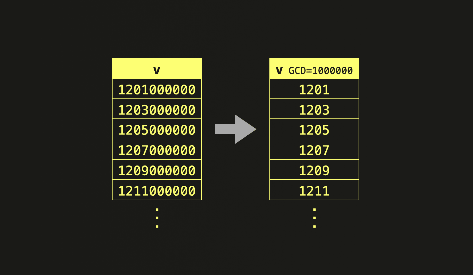
For example, taking the first row in the diagram above. The initial value is 1,201,000,000, which is stored as 1,201 with a GCD of 1,000,000. At query time the value 1,201 will be multiplied by 1,000,000 to get back to 1,201,000,000.
Reducing the scale of the values also has the added benefit of increasing the opportunity for other codecs, such as Delta, to further compress the data. Even general-purpose algorithms such as LZ4 and ZSTD can benefit from this reduction in range.
As an example, to show the potential benefits of the GCD codec, we use a 11+ billion row Forex dataset below. This dataset contains two Decimal columns, the bid and ask, for which we assess the impact of the GCD codec on compression for the following table configurations:
forex_v1-Decimal(76, 38) CODEC(ZSTD)- The precision and scale here are much larger than required, causing thebidandaskto be stored in a larger integer representation than needed. ZSTD compression is applied.forex_v2-Decimal(76, 38) CODEC(GCD, ZSTD)- Same as the above but with the GCD codec applied before ZSTD compression.forex_v3-Decimal(11, 5) CODEC(ZSTD)- The optimal (minimal) precision and scale for the values. ZSTD compression is applied.forex_v4-Decimal(11, 5) CODEC(GCD, ZSTD)- The optimal precision and scale for the values with the GCD codec and ZSTD.
*ZSTD(1) in all cases.
Note: internally Decimal numbers are stored as normal signed integers with the precision determining the bits required.
The example table schema and data load are shown below:
CREATE TABLE forex
(
	`datetime` DateTime64(3),
	`bid` Decimal(11, 5) CODEC(ZSTD(1)),
	`ask` Decimal(11, 5) CODEC(ZSTD(1)),
	`base` LowCardinality(String),
	`quote` LowCardinality(String)
)
ENGINE = MergeTree
ORDER BY (base, quote, datetime)

INSERT INTO forex
SELECT *
FROM s3Cluster('default', 'https://datasets-documentation.s3.eu-west-3.amazonaws.com/forex/csv/year_month/*.csv.zst', 'CSVWithNames')
SETTINGS min_insert_block_size_rows = 10000000, min_insert_block_size_bytes = 0, parts_to_throw_insert = 50000, max_insert_threads = 30, parallel_distributed_insert_select = 2
We can inspect the compression for the bid and ask columns for each table configuration with the following query:
SELECT
	table,
	name,
	any(compression_codec) AS codec,
	any(type) AS type,
	formatReadableSize(sum(data_compressed_bytes)) AS compressed_size,
	formatReadableSize(sum(data_uncompressed_bytes)) AS uncompressed_size,
	round(sum(data_uncompressed_bytes) / sum(data_compressed_bytes), 2) AS ratio
FROM system.columns
WHERE (table LIKE 'forex%') AND (name IN ['bid', 'ask'])
GROUP BY
	table,
	name
ORDER BY
	table ASC,
	name DESC

┌─table────┬─name─┬─codec───────────────┬─type───────────┬─compressed_size─┬─uncompressed_size─┬─ratio─┐
│ forex_v1 │ bid  │ CODEC(ZSTD(1))  	│ DECIMAL(76, 38)│ 23.56 GiB   	   │ 345.16 GiB    	   │ 14.65 │
│ forex_v1 │ ask  │ CODEC(ZSTD(1))  	│ DECIMAL(76, 38)│ 23.61 GiB   	   │ 345.16 GiB    	   │ 14.62 │
│ forex_v2 │ bid  │ CODEC(GCD, ZSTD(1)) │ DECIMAL(76, 38)│ 14.47 GiB   	   │ 345.16 GiB    	   │ 23.86 │
│ forex_v2 │ ask  │ CODEC(GCD, ZSTD(1)) │ DECIMAL(76, 38)│ 14.47 GiB   	   │ 345.16 GiB    	   │ 23.85 │
│ forex_v3 │ bid  │ CODEC(ZSTD(1))  	│ DECIMAL(11, 5) │ 11.99 GiB   	   │ 86.29 GiB     	   │   7.2 │
│ forex_v3 │ ask  │ CODEC(ZSTD(1))  	│ DECIMAL(11, 5) │ 12.00 GiB   	   │ 86.29 GiB     	   │  7.19 │
│ forex_v4 │ bid  │ CODEC(GCD, ZSTD(1)) │ DECIMAL(11, 5) │ 9.77 GiB    	   │ 86.29 GiB     	   │  8.83 │
│ forex_v4 │ ask  │ CODEC(GCD, ZSTD(1)) │ DECIMAL(11, 5) │ 9.78 GiB    	   │ 86.29 GiB     	   │  8.83 │
└──────────┴──────┴─────────────────────┴────────────────┴─────────────────┴───────────────────┴───────┘
Clearly, defining a column with unnecessarily high precision and scale has significant consequences on the compressed and uncompressed size, with forex_v1 occupying almost twice as much space as the nearest other configurations at 23.56 GiB While GCD will not impact the uncompressed size, it does reduce the compressed size by 38% to 14.47GiB. GCD is, therefore, useful in cases where the precision used is higher than necessary.
These results also show that specifying the right precision and scale can offer dramatic improvements with forex_v3 consuming only 12 Gib. The reduction in uncompressed size, which is only a1/4 of the size, is more predictable due to the lower number of bits used for each value '64 vs 256`.
Finally, even with an optimized precision and scale, the GCD codec provides significant compression improvements here. We have reduced the compressed size of our columns by almost 20% to 9.8GiB.
This hopefully shows the potential for the GCD codec. Let us know if it's useful and the savings you've made!
Simple authentication with SSH Keys
Contributed by George Gamezardashvili
Data engineers and database administrators logging into many ClickHouse clusters, each time with a different password, will hopefully appreciate this feature. ClickHouse now supports the ability to authenticate via an SSH key. This simply requires the user to add their public key to the ClickHouse configuration file.
$ cat users.d/alexey.yaml

users:
  alexey:
	ssh_keys:
  	ssh_key:
    	type: ssh-rsa
    	# cat ~/.ssh/id_rsa.pub
    	base64_key: 'AAAAB3NzaC1yc2EAAAABIwAAAQEAoZiwf7tVzIXGW26cuqnu...'
or via DDL
CREATE USER alexey IDENTIFIED WITH ssh_key BY KEY 'AAAAB3NzaC1yc2EAAAABIwAAAQEAoZiwf7tVzIXGW26cuqnu...' TYPE 'ssh-rsa'
When connecting to a ClickHouse server, instead of providing a password, the user specifies the path to their private key.
$ clickhouse-client --ssh-key-file ~/.ssh/id_rsa --user alexey
Needing to provide the path to your SSH key each time might be frustrating for some users, especially if connecting to multiple servers. Don’t forget that you can also configure client settings via configuration. This file is located in your home directory i.e. ~/.clickhouse-client/config.xml. The above settings can be configured as follows:
<?xml version="1.0" ?>
<config>
    <secure>1</secure>
    <host>default_host</host>
    <openSSL>
   	 <client>
   		 <loadDefaultCAFile>true</loadDefaultCAFile>
   		 <cacheSessions>true</cacheSessions>
   		 <disableProtocols>sslv2,sslv3</disableProtocols>
   		 <preferServerCiphers>true</preferServerCiphers>
   		 <invalidCertificateHandler>
   			 <name>RejectCertificateHandler</name>
   		 </invalidCertificateHandler>
   	 </client>
    </openSSL>
    <prompt_by_server_display_name>
   	 <default>{display_name} :) </default>
    </prompt_by_server_display_name>
	<!--Specify private SSH key-->
	<user>alexey</user>
	<ssh-key-file>~/.ssh/id_rsa</ssh-key-file>
</config>
Provided your public key has been distributed to our ClickHouse instance configurations, you can connect without needing to specify the location of your public key.
clickhouse-client --host <optional_host_if_not_default>
Note: users will be prompted for a passphrase when using an SSH key. This can either be entered in response or configured via the parameter --ssh-key-passphrase.
For our cloud users, we're working on making this available as soon as possible.
Workload scheduling - The foundations of something bigger
Contributed by Sergei Trifonov
One of the most anticipated features of ClickHouse is the ability to isolate query workloads. More specifically, users often need to define the resource limits for a set of queries with the intention of minimizing their impact. The goal here is often to ensure these queries do not impact other business-critical queries.
For example, a ClickHouse administrator may need to run a large query, which is expected to consume significant resources and take minutes, if not hours, to complete. During this query execution, ClickHouse has to continue to serve fast queries from a business-critical application. Ideally, the long-running query would be executed in such a way that the smaller critical fast queries were not impacted.
While this is partially possible with memory quotas and CPU limits in ClickHouse, we acknowledge it currently is not as easily achieved as it should be. There is also no means to limit the usage of shared resources such as disk I/O.
We are therefore pleased to announce the foundations of Workload scheduling.
While the initial implementation of this feature focuses on being able to schedule remote disk IO, it includes the framework and foundation to which other resources can be added.
Once a workload is created, queries can, in turn, be scheduled with a workload SETTING e.g.
SELECT count() FROM my_table WHERE value = 42 SETTINGS workload = 'long_running_limited'
SELECT count() FROM my_table WHERE value = 42 SETTINGS workload = 'priority'
For full details on how to configure workload schedules, we recommend the documentation.