Table of Contents
- Introduction
- Choosing ClickHouse
- The scale of the problem
- ClickHouse Cloud infrastructure
- Building on top of ClickHouse Cloud
- Understanding your users
- Some early design decisions
- Choosing OpenTelemetry (OTel)
- Architectural overview
- Ingest processing
- Schema
- Enhancing Grafana
- Cross-region querying
- Performance and cost
- Looking forward
- Conclusion
Introduction
We believe in dogfooding our own technologies wherever possible, especially when it comes to addressing challenges we believe ClickHouse solves best. Last year, we explained in detail how we used ClickHouse to build an internal data warehouse and the challenges we faced. In this post, we explore a different internal use case: observability and how we use ClickHouse to address our internal requirements and store the enormous volumes of log data generated by ClickHouse Cloud. As you’ll read below, this saves us millions of dollars a year and allows us to scale out our ClickHouse Cloud service without having to be concerned about observability costs, or make compromises on the log data we retain.
In the interest of others benefiting from our journey, we provide the details of our own ClickHouse-powered logging solution that contains over 19 PiB uncompressed, or 37 trillion rows, for our AWS regions alone. As a general design philosophy, we aspired to minimize the number of moving parts and ensure the design was as simple and reproducible as possible.
As we show later in our pricing analysis section, ClickHouse is at least 200x less expensive than Datadog for our workload, assuming Datadog and AWS list prices for hosting ClickHouse and storing data in S3.
A small team with an enormous challenge
When we first released our initial offering of ClickHouse Cloud over a year ago, we had to make compromises. While we recognized that ClickHouse could be used to build an observability solution at the time, our priority was to build the Cloud service itself. Laser-focused on delivering a world-class service as soon as possible, we initially decided to use Datadog as a recognized market leader in cloud observability to speed up time-to-market.
While this allowed us to get ClickHouse Cloud to GA quickly, it became apparent the Datadog bill would become an unsustainable cost. As ClickHouse server and Keeper logs comprise 98% of the log data we collect, our data volumes effectively grow linearly to the number of clusters we deploy.
Our initial response to this challenge was to do what most Datadog users are probably forced to do – consider limiting data retention times to reduce costs. While limiting the data retention to 7 days can be an effective means to control costs, it was in direct conflict with the needs of our users (our core and support engineers investigating issues) and the primary objective of providing a first-class service. Should an issue be identified in ClickHouse (yes, we have bugs), our core engineers need to be able to search all logs across all clusters for a period of up to 6 months.
For a 30-day retention period (a long way off our 6-month requirement), before any discounts, Datadog's list pricing of $2.5 per million events and $0.1 per GB ingested (assuming an annual contract) meant a monthly projected cost of $26M for our current 5.4 PiB/10.17 trillion rows per month. And at the required 6-months retention, well, let's just say it wasn't considered.
Choosing ClickHouse
With the experience of operating ClickHouse at scale, knowing that it would be significantly cheaper for the same workload, as well as having seen other companies already build their logging solutions on ClickHouse (e.g., highlight.io and Signoz) we prioritized the migration of the storage of our log data to ClickHouse and formed an internal Observability team. With a small team of 1.5 full-time engineers, we set about building our ClickHouse-powered logging platform “LogHouse” in under three months!
Our Internal Observability team is responsible for more than just LogHouse. With a wider remit to enable engineers at ClickHouse to understand what is going on with all of the clusters in ClickHouse Cloud that we are running, we provide a number of services, including an alerting service, for detecting patterns of cluster behavior that should be proactively addressed.
The scale of the problem
ClickHouse Cloud is available in 9 AWS and 4 GCP regions as of the time of writing, with Azure support coming soon. Our largest region alone produces over 1.1 million log lines per second. Across all AWS regions, this creates some eye-watering numbers:
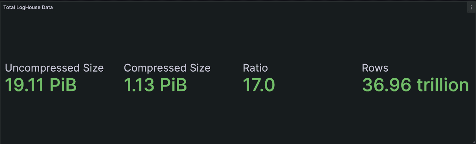
What might be immediately apparent here is the compression level we achieve - 19 PiB compresses to around 1.13 PiB, or 17x compression. This level of compression achieved by ClickHouse was critical to the success of the project and allowed us to scale cost efficiently while still delivering good query performance.
Our total LogHouse environment currently exceeds 19 PiB. This figure accounts for our AWS environment alone.
ClickHouse Cloud infrastructure
We’ve discussed the architecture behind ClickHouse Cloud in previous posts. The principal feature of this architecture that is relevant to our logging solution is that ClickHouse instances are deployed as pods in Kubernetes and orchestrated by a custom operator.
Pods log to stdout and stderr and are captured by Kubernetes as files per the standard configuration. An OpenTelemetry agent can then read these log files and forward them to ClickHouse.
While the majority of our data originates from ClickHouse servers (some instances can log 4,000 lines per second under heavy load) and Keeper logs, we also collect data from the cloud data plane. This consists of logs from our operator and supporting services running on nodes. For ClickHouse cluster orchestration, we rely on ClickHouse Keeper (a C++ ZooKeeper alternative developed by our core team), which produces detailed logs involving cluster operations. While the Keeper logs compromise around 50% of traffic at any moment (vs 49% for ClickHouse server logs and 1% from the data plane), the retention for this dataset is shorter at 1 week (vs 6 months for server logs), meaning it represents a much smaller percentage of the overall data.
Building on top of ClickHouse Cloud
Since we are monitoring ClickHouse Cloud, the cluster powering LogHouse could not live within the ClickHouse Cloud infrastructure itself – otherwise, we would be creating a dependency between the system being monitored and the monitoring tool.
However, we still wanted to benefit from the technology behind ClickHouse Cloud – specifically, the separation of storage and compute through the SharedMergeTree table engine. Principally, this allows us to benefit from storing our data in S3 with large NVMe caches locally, and allows us to scale our clusters almost infinitely wide. Given our volumes, which will only increase as we onboard more customers, we did not want to incur the challenge of having to provision more clusters and/or nodes due to disk space limitations. By storing all data in S3, with nodes only using local NVMe for cache, we could scale easily and focus on the data itself.
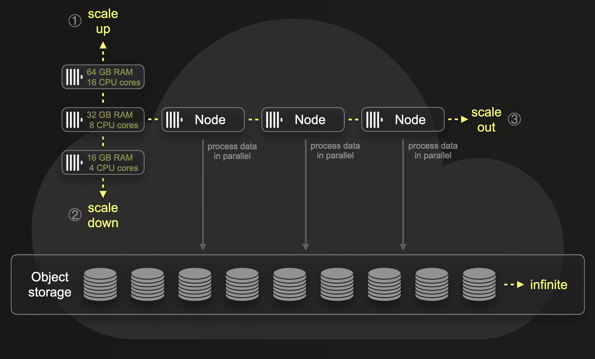
We, therefore, run our own "mini ClickHouse Cloud" in each region (see below), even using ClickHouse Cloud's Kubernetes operator. The ability to use "cloud" was fundamental to us being able to build the solution in such a short period of time, and manage the infrastructure with a small team. We truly are standing on the shoulders of giants (aka the ClickHouse core team).
While this solution is specific to our needs, it is equivalent to ClickHouse Cloud’s Dedicated Tier offering, where a customer’s cluster is deployed on dedicated infrastructure, allowing them to control aspects of the deployment, such as update and maintenance windows. Most importantly, other users wanting to replicate our solution would not be subject to the same circular dependency constraints and could simply use a ClickHouse Cloud cluster.
We are currently working on moving internal clusters (like LogHouse) into our ClickHouse Cloud infrastructure. Where it will be isolated in a separate Kubernetes cluster but will otherwise be a "standard" ClickHouse Cloud cluster identical to what our customers use.
Understanding your users
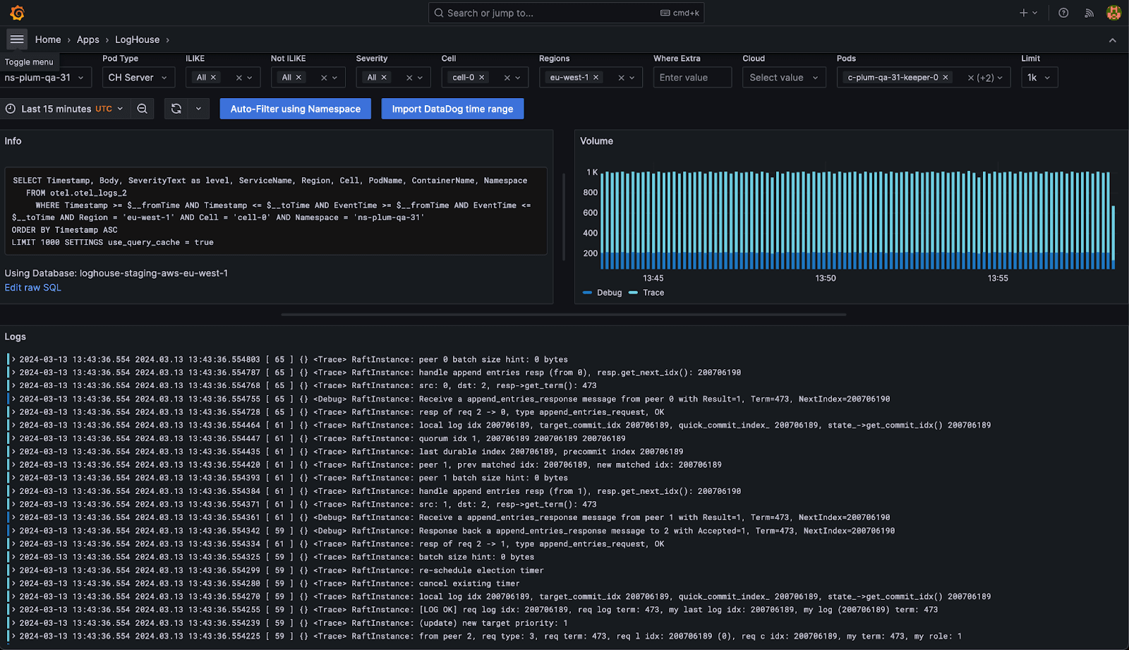
Using ClickHouse for log storage requires users to embrace SQL-based Observability. Principally, this means users are comfortable searching for logs using SQL and ClickHouse’s large set of string matching and analytical functions. This adoption is made simpler with visualization tools such as Grafana, which provides query builders for common observability operations.
In our case, our users are deeply familiar with SQL as ClickHouse support and core engineers. While this has the benefit that queries are typically heavily optimized, it introduces its own set of challenges. Most notably, these users are power users, who will use visual-based tooling for initial analysis only, before wanting to connect directly to LogHouse instances via the ClickHouse client. This means we need an easy way for users to easily navigate between any dashboard and the client.
In most cases, investigations into Cloud issues are initiated by alerts triggered from cluster metrics collected by Prometheus. These detect potentially problematic behaviors (e.g. a large number of parts), which should be investigated. Alternatively, a customer may raise an issue through support channels indicating an unusual behavior or unexplainable error.
Logs become relevant to an investigation once this deeper analysis is required. By this point, our support or core engineers have therefore identified the customer cluster, its region, and the associated Kubernetes namespace. This means most searches are filtered by both time and a set of pod names – the latter of these can be identified from the Kubernetes namespace easily.
The schemas we show later are optimized for these specific workflows and contribute to being able to deliver excellent query performance at multi-petabyte scale.
Some early design decisions
The following early design decisions heavily influenced our final architecture.
No data sent across regions
Firstly, we do not send log data across regions. Given the volumes even small regions produce, centralizing logging was not viable from the data egress cost perspective. Instead, we host a LogHouse cluster in each region. As we will discuss below, users can still query across regions.
No Kafka queue as a message buffer
Using a Kafka queue as a message buffer is a popular design pattern seen in logging architectures and was popularized by the ELK stack. It provides a few benefits; principally, it helps provide stronger message delivery guarantees and helps deal with backpressure. Messages are sent from collection agents to Kafka and written to disk. In theory, a clustered Kafka instance should provide a high throughput message buffer, since it incurs less computational overhead to write data linearly to disk than parse and process a message – in Elastic, for example, the tokenization and indexing incurs significant overhead. By moving data away from the agents, you also incur less risk of losing messages as a result of log rotation at the source. Finally, it offers some message reply and cross-region replication capabilities, which might be attractive for some use cases.
However, ClickHouse can handle inserting data very, very quickly – millions of rows per second on moderate hardware. Back pressure from ClickHouse is rare**.** Thus, at our scale, leveraging a Kafka queue simply did not make sense and meant more architectural complexity and cost than was necessary. In settling on this architecture, we also embrace an important principle – not all logs require the same delivery guarantees. In our case, our tolerance for in-transit data drops is higher, as there is a second copy of the logs (on the instances themselves) should we need them - although, we still look to minimize any in-transit data drops as missing messages have the potential to disrupt investigations.
Improving in-transit data drops
We currently have higher in-transit drop rates than we are comfortable with. We attribute this to several factors:
- Lack of autoscaling in our ingestion layer, which can be vulnerable to spikes of traffic when specific events are initiated in ClickHouse Cloud (e.g. an update). Despite (2), this is a feature we intend to develop.
- We have identified an issue in the OTEL collector where connections between the agents and gateways are not evenly distributed, causing “hotspots” to occur at the gateways where a single collector receives a higher percentage of the load. This collector becomes overwhelmed, and when combined with (1), we experience increased rates of logs being dropped in-transit. We are resolving this issue and intend to contribute the fix back so others can benefit.
We are not currently utilizing the auto-scaling capabilities of ClickHouse Cloud, as instances of backpressure from ClickHouse itself are infrequent. However, as we address and resolve the preceding issues, our ClickHouse instances may experience increased traffic spikes. Up until now, existing challenges with the collector have acted as a buffer, shielding ClickHouse from such fluctuations. Moving forward, we may thus need to explore the potential benefits of implementing ClickHouse Cloud's auto-scaler to better manage these expected increases in demand.
Despite these challenges, we do not regret our decision not to deploy Kafka. By embracing this principle, our resulting architecture is simpler, cheaper, and lower latency, and we are confident we can reduce the rates of in-transit data drops to an acceptable level by taking the actions described above.
Structured logging
We would like to say that our logs were always structured and cleanly inserted into a perfect schema. However, that is not the case. Our initial deployment sent logs as a plaintext string, with users relying on ClickHouse string functions to extract metadata. This was motivated by a preference of our users to consume the logs in their original form. While this still offered great compression, query performance suffered since every query incurred a linear scan. This was an original architectural mistake which we encourage you not to repeat.
After discussing the pros and cons with our users, we moved to structured logging, with ClickHouse instances logging in JSON. As described below, these JSON keys are stored in a Map(String, String) type by default. However, select fields on which we expect frequent queries are extracted at insert time as full columns. These can then be used in our ordering key and configured to exploit secondary indices and specialized codecs. This allows queries on columns such as pod_name to be optimized, ensuring the most common workflows are optimized for query performance. Users can still access Map keys for less frequently accessed metadata. However, in our experience, this is rarely done without a filter on an optimized column.
Choosing OpenTelemetry (OTel)
The decision to use OpenTelemetry was our biggest design decision and thus deserves its own section. This also represented the decision we were initially most nervous about since the ClickHouse OTel exporter was relatively unproven for log collection (compared to tracing) when we started the project - it was in alpha, and we were not aware of any deployments at our scale. Our decision to invest was based on a number of factors:
- Community adoption - The wider OTel project has seen remarkable adoption. We also saw other companies using the ClickHouse exporter successfully despite its alpha status. Furthermore, a number of ClickHouse-powered Observability companies, such as highlight.io and Signoz, use OTel as their standard for ingestion.
- Investing in the future - The project itself has reached a level of maturity and adoption, which suggests it will become the de facto means of collecting logs, traces, and metrics. Investments by proprietary observability vendors such as Dynatrace, Datadog, and Splunk suggested a wider acceptance of its emergence as a standard.
- Looking beyond logs - We considered other log collection agents, specifically Fluentd and Vector, but wanted a stack that would allow us to easily expand LogHouse to collect metrics and traces later.
Custom processor
One of the common frustrations with OTel is the need to declare complex pipelines in YAML, linking receivers, processors, and senders. We perform a significant amount of processing in OTel collector instances (at a gateway layer - see below) with the need to perform conditional routing based on the source, e.g. ClickHouse instance, data plane, and Keeper logs all go to separate tables with optimized schemas.
In our experience, managing this YAML code was error-prone and tricky to test. Rather than relying on this, we developed a custom processor in Go that performs all of our required transformation logic. This means we deploy a custom build of the OTel collector, but we benefit from being able to test any changes to processing easily. This internal pipeline using a custom processor is also faster than the equivalent constructed from a declarative approach, further saving us resources and reducing end-to-end latency.
Architectural overview
At a high-level level, our pipeline looks like the following:
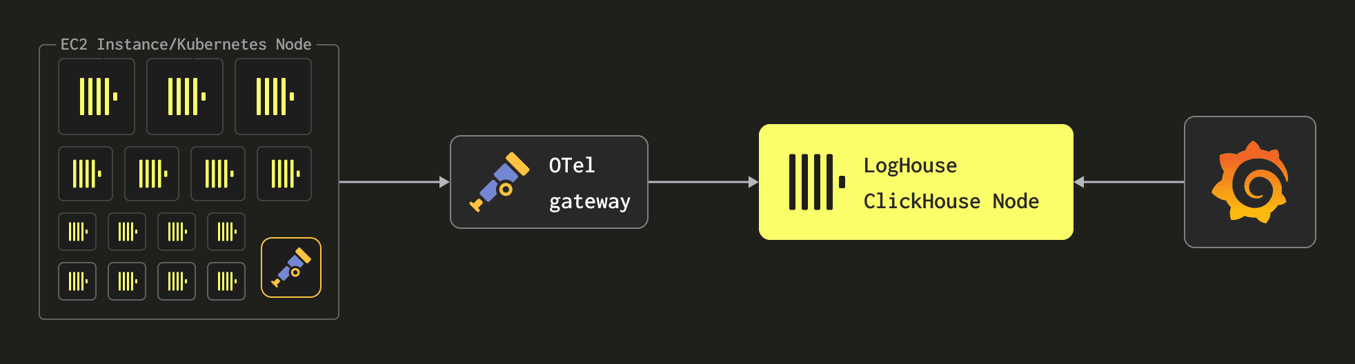
We deploy the OTel collector as both an agent on each Kubernetes node for log collection and as a gateway where messages are processed before being sent to ClickHouse. This is a classic agent-gateway architecture documented by Open Telemetry and allows the overhead of log processing to be moved away from the nodes themselves. This helps ensure the agent resource footprint is as minimal as possible since it is only responsible for forwarding logs to a gateway instance. As gateways perform all message processing, these must also be scaled as the number of Kubernetes nodes and, thus, logs increase. As we’ll show below, this architecture leaves us with an agent per node whose resources are assigned based on the underlying instance type. This is based on the reasoning that larger instance types have more ClickHouse activity and, thus, more logs. These agents then forward their logs to a “bank” of gateways for processing, which are scaled based on total log throughput.
Expanding on the above, a single region, either AWS or GCP (and soon to be Azure), can look something like the following:

What should be immediately apparent is how architecturally simple this is. A few important notes with respect to this:
- Our ClickHouse Cloud environment (AWS) currently uses a mixture of
m5d.24xlarge(96 vCPUs, 384GiB RAM),m5d.16xlarge(64 vCPUs, 256GiB RAM),m5d.8xlarge(32 vCPUs, 128GiB RAM),m5d.2xlarge(8 vCPUs, 32GiB RAM), andr5d.2xlarge(8 vCPU 64GiB). Since ClickHouse Cloud allows users to create clusters of varying total resource size (a fixed 1:4 vCPU:RAM ratio is used), through vertical and horizontal scaling, the actual size of ClickHouse pods can vary. How these are packed onto the nodes is a topic in itself but we recommend this blog. In general, however, this means larger instance types host more ClickHouse pods (which generate most of our log data). This means there is a strong correlation between instance size and the amount of log data generated that needs to be forwarded by an agent. - OTel Collector agents are deployed as daemonsets on each Kubernetes node. The resources assigned to these depend on the underlying instance size. In general, we have three t-shirt sizes of varying resources: small, medium, or large. For a
m5d.16xlargeinstance, we utilize a large agent, which is assigned 1vCPU and 1GiB of memory. This is sufficient to deal with collecting the logs from ClickHouse instances on this node even when the node is fully occupied. We perform minimal processing at the agent level to minimize resource overhead, only extracting the timestamp from the log file to override the Kubernetes observed timestamp. Assigning higher resources to agents would have implications beyond the cost of their hosting. Importantly, they can impact our operator's ability to pack ClickHouse instances efficiently on the node, potentially causing evictions and underutilized resources. The following shows the mapping from node size to agent resources (AWS only):
| Kubernetes Node Size | Collector agent T-shirt size | Resources to collector agent | Logging rate |
|---|---|---|---|
| m5d.16xlarge | Large | 1 CPU, 1GiB | 10k/second |
| m5d.8xlarge | Medium | 0.5 CPU, 0.5GiB | 5k/second |
| m5d.2xlarge | Small | 0.2CPU, 0.2GiB | 1k/second |
- OTel collector agents send their data to gateway instances via a Kubernetes service configured to use topology-aware routing. Since each region has at least one gateway in each availability zone (for high availability), this ensures data by default is routed to the same AZ if possible. In larger regions, where log throughput is higher, we provision more gateways to handle the load. For example, in our largest region, we currently have 16 gateways to handle the 1.1M rows/sec. Each of these has 11 GiB of RAM and three cores.
- Since our LogHouse instances reside in a different Kubernetes cluster, to maintain isolation from Cloud, gateways forward their traffic to these ClickHouse instances via an NLB for the cluster. This is currently not zone-aware and results in higher inter-zone communication than optimal. We are thus in the process of ensuring this NLB exploits the recently announced Availability Zone DNS affinity.
- Our gateway and agents are all deployed by Helm charts, which are deployed automatically as part of a CI/CD pipeline orchestrated by ArgoCD with configuration in Git.
- Our collector gateways are monitored via Prometheus metrics, with alerts indicating when these experience resource pressure.
- Our ClickHouse instances use an identical deployment architecture to Cloud - 3 Keeper instances spread across different AZs, with ClickHouse also distributed accordingly.
- Our largest LogHouse ClickHouse cluster consists of 5 nodes, each 200GiB RAM and 57 cores deployed on an
m5d.16xlarge. This handles over 1M row inserts per second. - A single instance of Grafana is currently deployed per region, with its traffic load balanced across its local LogHouse cluster via the NLB. As we discuss in more detail below, however, each Grafana is able to access other regions (via TailScale VPN and IP whitelisting).
Tuning gateways and handling back pressure
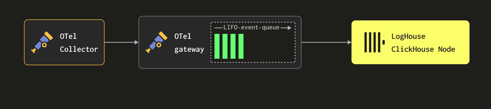
Given our gateways perform the majority of our data processing, obtaining performance from these is key to minimizing costs and maximizing throughput. During testing, we established that each gateway, with three cores, could handle around 60K events/sec.
Our gateways perform no disk persistence of data, buffering events only in memory. Currently, our gateways are assigned 11 GiB, with sufficient numbers deployed in each region to provide up to 2 hours of buffering in the rare event that ClickHouse becomes unavailable. Our current memory-to-CPU ratio and number of gateways are thus a compromise between throughput and providing sufficient memory to buffer log messages in the event ClickHouse becomes unavailable. We prefer to scale out gateways horizontally since it provides better fault tolerance (if some EC2 node experiences a problem, we are less at risk).
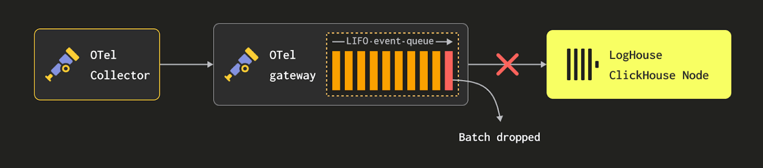
Importantly, if the buffers become full, events at the front of the queue will be dropped, i.e. gateways will always accept events from the agents themselves, where we apply no backpressure. However, our 2-hour window has proven sufficient, with OTel pipeline issues rarely impacting our data retention quality. That said, we are also currently exploring the ability of the OTel collector to buffer to disk for our gateways - thus potentially allowing us to provide greater resilience to downstream issues while also possibly reducing the memory footprint of the gateways.
We performed some rudimentary testing during initial deployment to establish an optimal batch size. This is a compromise between wanting to insert data into ClickHouse efficiently and ensuring logs are available in a timely manner for searches. More specifically, while larger batches are generally more optimal for inserts for ClickHouse, this has to be balanced against data being available and memory pressure on the gateways (and ClickHouse at very large batch sizes). We settled on a batch size of 15K rows for the batch processor, which delivered the throughput we needed and satisfied our data availability SLA of 2 minutes.
Finally, we do have periods of lower throughput. We, therefore, also flush the batch processor in the gateway after 5 seconds (see timeout) to ensure data is available within the above SLA. As this may result in smaller inserts, we adhere to ClickHouse's best practices and rely on asynchronous Inserts.
Ingest processing
Materialized views
The OTel collector collates fields into two primary maps: ResourceAttributes and LogAttributes. The former of these contains fields added by the agent instance and, in our case, mostly consists of Kubernetes metadata, such as the pod name and namespace. The LogAttributes field conversely contains the actual contents of the log message. As we log in structured JSON, this can contain multiple fields, e.g. the thread name and the source code line from which the log was produced.
{
  "Timestamp": "1710415479782166000",
  "TraceId": "",
  "SpanId": "",
  "TraceFlags": "0",
  "SeverityText": "DEBUG",
  "SeverityNumber": "5",
  "ServiceName": "c-cobalt-ui-85-server",
  "Body": "Peak memory usage (for query): 28.34 MiB.",
  "ResourceSchemaUrl": "https://opentelemetry.io/schemas/1.6.1",
  "ScopeSchemaUrl": "",
  "ScopeName": "",
  "ScopeVersion": "",
  "ScopeAttributes": "{}",
  "ResourceAttributes": "{
      \"cell\":\"cell-0\",
      \"cloud.platform\":\"aws_eks\",
      \"cloud.provider\":\"aws\",
      \"cluster_type\":\"data-plane\",
      \"env\":\"staging\",
      \"k8s.container.name\":\"c-cobalt-ui-85-server\",
      \"k8s.container.restart_count\":\"0\",
      \"k8s.namespace.name\":\"ns-cobalt-ui-85\",
      \"k8s.pod.name\":\"c-cobalt-ui-85-server-ajb978y-0\",
      \"k8s.pod.uid\":\"e8f060c5-0cd2-4653-8a2e-d7e19e4133f9\",
      \"region\":\"eu-west-1\",
      \"service.name\":\"c-cobalt-ui-85-server\"}",
  "LogAttributes": {
      \"date_time\":\"1710415479.782166\",
      \"level\":\"Debug\",
      \"logger_name\":\"MemoryTracker\",
      \"query_id\":\"43ab3b35-82e5-4e77-97be-844b8656bad6\",
      \"source_file\":\"src/Common/MemoryTracker.cpp; void MemoryTracker::logPeakMemoryUsage()\",
      \"source_line\":\"159\",
      \"thread_id\":\"1326\",
      \"thread_name\":\"TCPServerConnection ([#264])\"}"
}
Importantly, the keys in either of these maps are subject to change and are semi-structured. For example, new Kubernetes labels could be introduced at any time. While the Map type in ClickHouse is great for collecting arbitrary key-value pairs, it does not provide optimal query performance. As of 24.2, a query on a Map column requires the entire map values to be decompressed and read - even if accessing a single key. We recommend that users use Materialized Views to extract the most commonly queried fields into dedicated columns, which is simple to do with ClickHouse, and dramatically improves query performance. For example, the above message might become:
{
  "Timestamp": "1710415479782166000",
  "EventDate": "1710374400000",
  "EventTime": "1710415479000",
  "TraceId": "",
  "SpanId": "",
  "TraceFlags": "0",
  "SeverityText": "DEBUG",
  "SeverityNumber": "5",
  "ServiceName": "c-cobalt-ui-85-server",
  "Body": "Peak memory usage (for query): 28.34 MiB.",
  "Namespace": "ns-cobalt-ui-85",
  "Cell": "cell-0",
  "CloudProvider": "aws",
  "Region": "eu-west-1",
  "ContainerName": "c-cobalt-ui-85-server",
  "PodName": "c-cobalt-ui-85-server-ajb978y-0",
  "query_id": "43ab3b35-82e5-4e77-97be-844b8656bad6",
  "logger_name": "MemoryTracker",
  "source_file": "src/Common/MemoryTracker.cpp; void MemoryTracker::logPeakMemoryUsage()",
  "source_line": "159",
  "level": "Debug",
  "thread_name": "TCPServerConnection ([#264])",
  "thread_id": "1326",
  "ResourceSchemaUrl": "https://opentelemetry.io/schemas/1.6.1",
  "ScopeSchemaUrl": "",
  "ScopeName": "",
  "ScopeVersion": "",
  "ScopeAttributes": "{}",
  "ResourceAttributes": "{
      \"cell\":\"cell-0\",
      \"cloud.platform\":\"aws_eks\",
      \"cloud.provider\":\"aws\",
      \"cluster_type\":\"data-plane\",
      \"env\":\"staging\",
      \"k8s.container.name\":\"c-cobalt-ui-85-server\",
      \"k8s.container.restart_count\":\"0\",
      \"k8s.namespace.name\":\"ns-cobalt-ui-85\",
      \"k8s.pod.name\":\"c-cobalt-ui-85-server-ajb978y-0\",
      \"k8s.pod.uid\":\"e8f060c5-0cd2-4653-8a2e-d7e19e4133f9\",
      \"region\":\"eu-west-1\",
      \"service.name\":\"c-cobalt-ui-85-server\"}",
  "LogAttributes": "{
      \"date_time\":\"1710415479.782166\",
      \"level\":\"Debug\",
      \"logger_name\":\"MemoryTracker\",
      \"query_id\":\"43ab3b35-82e5-4e77-97be-844b8656bad6\",
      \"source_file\":\"src/Common/MemoryTracker.cpp; void MemoryTracker::logPeakMemoryUsage()\",
      \"source_line\":\"159\",
      \"thread_id\":\"1326\",
      \"thread_name\":\"TCPServerConnection ([#264])\"}"
}
To perform this transformation, we exploit Materialized Views in ClickHouse. Rather than inserting our data into a MergeTree table, our gateways insert into a Null table. This table is similar to /dev/null in that it does not persist the data it receives. However, Materialized Views attached to it execute a SELECT query over blocks of data as they are inserted. The results of these queries are sent to target SharedMergeTree tables, which store the final transformed rows. We illustrate this process below:
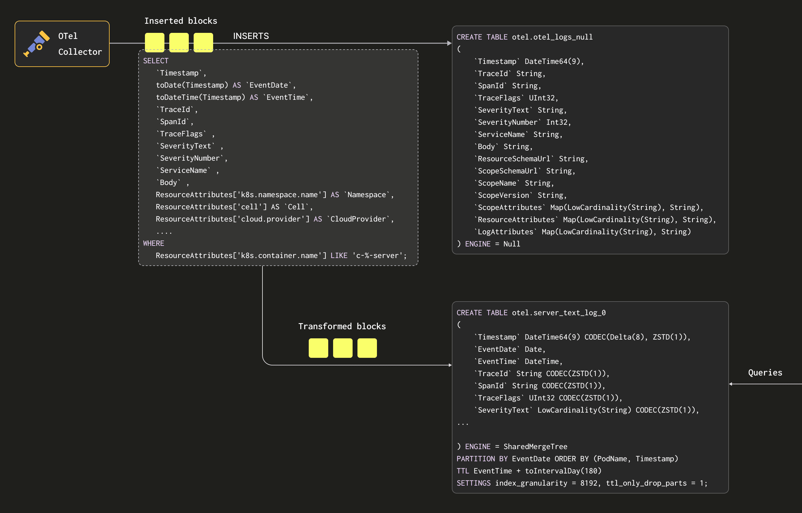
Using this mechanism, we have a flexible and native ClickHouse way to transform our rows. To change the schema and columns extracted from the map, we modify the target table before updating the view to extract the required columns.
Schema
Our data plane and Keeper logs have a dedicated schema. Given that the majority of our data is from ClickHouse server logs, we’ll focus on this schema below. This represents the target table that receives data from the Materialized Views:
CREATE TABLE otel.server_text_log_0
(
	`Timestamp` DateTime64(9) CODEC(Delta(8), ZSTD(1)),
	`EventDate` Date,
	`EventTime` DateTime,
	`TraceId` String CODEC(ZSTD(1)),
	`SpanId` String CODEC(ZSTD(1)),
	`TraceFlags` UInt32 CODEC(ZSTD(1)),
	`SeverityText` LowCardinality(String) CODEC(ZSTD(1)),
	`SeverityNumber` Int32 CODEC(ZSTD(1)),
	`ServiceName` LowCardinality(String) CODEC(ZSTD(1)),
	`Body` String CODEC(ZSTD(1)),
	`Namespace` LowCardinality(String),
	`Cell` LowCardinality(String),
	`CloudProvider` LowCardinality(String),
	`Region` LowCardinality(String),
	`ContainerName` LowCardinality(String),
	`PodName` LowCardinality(String),
	`query_id` String CODEC(ZSTD(1)),
	`logger_name` LowCardinality(String),
	`source_file` LowCardinality(String),
	`source_line` LowCardinality(String),
	`level` LowCardinality(String),
	`thread_name` LowCardinality(String),
	`thread_id` LowCardinality(String),
	`ResourceSchemaUrl` String CODEC(ZSTD(1)),
	`ScopeSchemaUrl` String CODEC(ZSTD(1)),
	`ScopeName` String CODEC(ZSTD(1)),
	`ScopeVersion` String CODEC(ZSTD(1)),
	`ScopeAttributes` Map(LowCardinality(String), String) CODEC(ZSTD(1)),
	`ResourceAttributes` Map(LowCardinality(String), String) CODEC(ZSTD(1)),
	`LogAttributes` Map(LowCardinality(String), String) CODEC(ZSTD(1)),
	INDEX idx_trace_id TraceId TYPE bloom_filter(0.001) GRANULARITY 1,
	INDEX idx_thread_id thread_id TYPE bloom_filter(0.001) GRANULARITY 1,
	INDEX idx_thread_name thread_name TYPE bloom_filter(0.001) GRANULARITY 1,
	INDEX idx_Namespace Namespace TYPE bloom_filter(0.001) GRANULARITY 1,
	INDEX idx_source_file source_file TYPE bloom_filter(0.001) GRANULARITY 1,
	INDEX idx_scope_attr_key mapKeys(ScopeAttributes) TYPE bloom_filter(0.01) GRANULARITY 1,
	INDEX idx_scope_attr_value mapValues(ScopeAttributes) TYPE bloom_filter(0.01) GRANULARITY 1,
	INDEX idx_res_attr_key mapKeys(ResourceAttributes) TYPE bloom_filter(0.01) GRANULARITY 1,
	INDEX idx_res_attr_value mapValues(ResourceAttributes) TYPE bloom_filter(0.01) GRANULARITY 1,
	INDEX idx_log_attr_key mapKeys(LogAttributes) TYPE bloom_filter(0.01) GRANULARITY 1,
	INDEX idx_log_attr_value mapValues(LogAttributes) TYPE bloom_filter(0.01) GRANULARITY 1,
	INDEX idx_body Body TYPE tokenbf_v1(32768, 3, 0) GRANULARITY 1
)
ENGINE = SharedMergeTree
PARTITION BY EventDate
ORDER BY (PodName, Timestamp)
TTL EventTime + toIntervalDay(180)
SETTINGS index_granularity = 8192, ttl_only_drop_parts = 1;
A few observations about our schema:
- We use the ordering key
(PodName, Timestamp). This is optimized for our query access patterns where users usually filter by these columns. Users will want to modify this based on their expected workflows. - We use the
LowCardinality(String) type for all String columns with the exception of those with very high cardinality. This dictionary encodes our string values and has proven to improve compression, and thus read performance. Our current rule of thumb is to apply this encoding for any string columns with a cardinality lower than 10,000 unique values. - Our default compression codec for all columns is ZSTD at level 1. This is specific to the fact our data is stored on S3. While ZSTD can be slower at compression when compared to alternatives, such as LZ4, this is offset by better compression ratios and consistently fast decompression (around 20% variance). These are preferable properties when using S3 for storage.
- Inherited from the OTel schema, we use
bloom_filtersfor the keys for any maps and values. This provides a secondary index on the keys and values of the maps based on a Bloom filter data structure. A Bloom filter is a data structure that allows space-efficient testing of set membership at the cost of a slight chance of false positives. In theory, this allows us to evaluate quickly whether granules on disk contain a specific map key or value. This filter might make sense logically as some map keys and values should be correlated with the ordering keys of pod name and timestamp i.e. the specific pods will have specific attributes. However, others will exist for every pod - we don’t expect these queries to be accelerated when querying on these values as the chances of the filtering condition being met by at least one of the rows in a granule is very high (in this configuration a block is a granule asGRANULARITY=1). For further details on why a correlation is needed between the ordering key and column/expression, see here. This general rule has been considered for other columns such asNamespace. Generally, these Bloom filters have been applied liberally and need to be optimized - a pending task. The false-positive rate of 0.01 has also not been tuned.
Expiring data
All of the schemas partition data by EventDate to provide a number of benefits - see the PARTITION BY EventDate in the above schema. Firstly, since most of our queries are over the last 6 hrs of data, this provides a quick way to filter to relevant parts. While this may mean the number of parts to query is higher on wider date ranges, we have not found this has appreciably impacted these queries.
Most importantly, it allows us to expire data efficiently. We can simply drop any partitions that exceed the retention time using ClickHouse’s core data management capabilities - see the TTL EventTime + toIntervalDay(180) declaration. For ClickHouse server logs, this is 180 days, as shown in the above schema, since our core team uses this to investigate the historical prevalence of any discovered issues. Other log types, such as those from Keeper, have much shorter retention needs as they serve less purpose beyond initial issue resolution. This partitioning means we can also use ttl_only_drop_parts for efficient dropping of data.
Enhancing Grafana
Grafana is our recommended visualization tool for observability data with ClickHouse. The recent version 4.0 release has made it much simpler to quickly query logs from the Explore view and is internally appreciated by our engineers. While we do use the plugin out of the box, we have also extended Grafana to meet our needs through an additional scenes plugin. This app, which we call LogHouse UI, is heavily opinionated and optimized for our specific workloads and integrates tightly with the Grafana Plugin. A few requirements motivated us to build this:
- There are specific visualizations that we always need to show for diagnostic purposes. While these could be supported through a dashboard, we want them to be tightly integrated with our log exploration experience - think of a hybrid of Explore and Dashboards. Dashboards would require the use of variables, which we find a little unwieldy at times, and we want to ensure our queries are as optimized as possible for the most common access patterns.
- Our users usually query with a namespace or cluster id when dealing with issues. The LogHouse UI is able to automatically limit this to query by pod name (and any user time restriction), thus ensuring our ordering keys are efficiently used.
- Given we have dedicated schemas for different data types, the LogHouse UI plugin automatically switches between backing schemas based on the query to provide a seamless experience for the user.
- Our actual table schemas are subject to change. While in most cases, we are able to make these modifications without affecting the UI, it helps that the interface is schema-aware. Our plugin, therefore, ensures it uses the right schema when querying specific time ranges. This allows us to make schema changes without concern of ever disrupting our user experience.
- Our users are highly proficient in SQL and often like to switch to query log data from the ClickHouse client after an initial investigation in the UI. Our application provides a clickhouse-client shortcut with the relevant SQL for any visualization. This allows our users to switch with a click between the respective tools, with typical workflows starting in Grafana before a deeper analysis is performed by connecting via the client, where highly focused SQL queries can be formulated.
- Our application has also enabled cross-region querying, as we’ll explore below.
Generally, most of our workload in relation to log data is explorative, with dashboards typically based on metric data. A custom log exploration experience, therefore, made sense and has proven worth the investment.
Cross-region querying
Always aspiring to provide the best experience possible for our users, we wanted to provide a single endpoint from which any ClickHouse cluster could be queried rather than users needing to navigate to region-specific Grafana instances to query the local data.
As we noted earlier, our data volumes are simply too large for any cross-region replication of data - the data egress charges alone would exceed the current costs of running our ClickHouse infrastructure. We, therefore, need to ensure that any ClickHouse cluster can be queried from the region in which Grafana is hosted (and its respective failover region).
Our initial naive implementation of this simply used a Distributed table in ClickHouse, so all regions could be queried from any node. This requires us to configure a logical cluster in every LogHouse region consisting of a shard for each region containing the respective nodes. This effectively creates a single monolithic cluster connecting to all LogHouse nodes in all regions.
While this works, a request must be issued to every node when the Distributed table is queried. Since we don’t replicate data across regions, only the nodes in one region have access to the relevant data for each query. This lack of geo-awareness means the other clusters expend resources evaluating a query that can never match. For queries that include a filter on the ordering key (pod name), this incurs a very small overhead. Broader, more investigative queries, however, especially involving linear scans, waste significant resources.
We were able to address this via clever use of the cluster function, but it made our queries rather unwieldy and unnecessarily complex. Instead, we utilize Grafana and our custom plugin to perform the required routing and make our application region-aware.
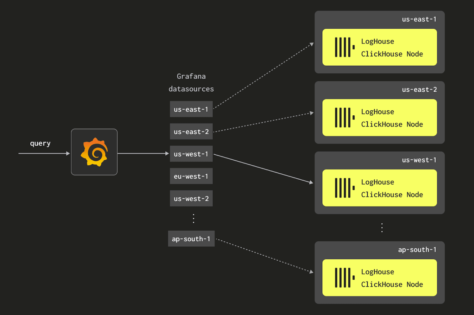
This requires every cluster to be configured as a data source. When a user queries for a specific namespace or pod, the custom plugin we built ensures only the data source associated with the pod's region is queried.
Performance and cost
Cost analysis
The following analysis does not consider our GCE infrastructure for LogHouse, and focuses exclusively on AWS. Our GCE environment does have similar linear price characteristics to that of AWS, with some variability in infrastructure costs.
Our current AWS LogHouse infrastructure costs $125k/month (at list price) and handles 5.4PiB throughput per month (uncompressed).
This $125,000 includes the hardware hosting our gateways. We note that these gateways also handle our metrics pipelines and are thus not dedicated to log processing. This number is therefore an overestimate as the hardware associated with LogHouse ingestion.
This infrastructure stores six months of data totaling 19 PiB uncompressed as just over 1 PiB of compressed data stored in S3. While it is hard for us to provide an exact cost model, we project our costs based on TiB throughput per month. This requires a few assumptions:
- Our EC2 infrastructure will scale linearly based on throughput. We are confident our OTel gateways will scale linearly with respect to resources and events per second. Larger throughputs will require more ClickHouse resources for ingestion. Again, we assume this is linear. Conversely, small throughputs will require less infrastructure.
- ClickHouse maintains a compression ratio of approximately 17x for our data.
- We assume our number of users is constant if our volumes grow and ignore S3 GET request charges – these are a function of queries and inserts and are not considered significant.
- We assume 30 days retention for simplicity.
In our most recent month we ingested 5532TB of data. Using this and the above cost we can compute our EC2 cost per TiB per month:
EC2 cost per TiB per month is ($125,000/5542) = $22.55
Using a cost per GiB in S3 of $0.021 and a compression ratio of 17x, this gives us a function:
T = TiB per month throughput (uncompressed)
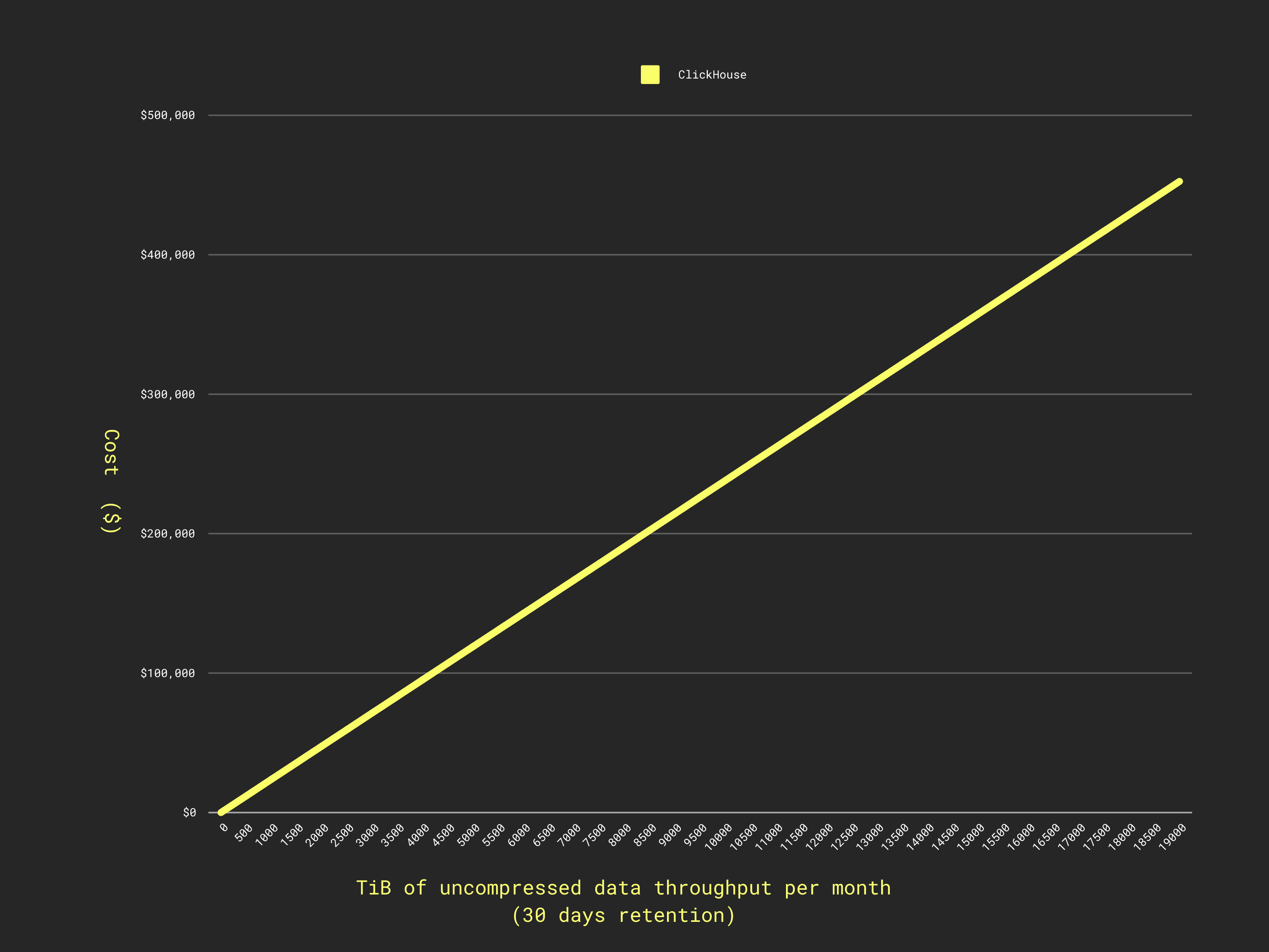
Cost ($) = EC2 Cost (Ingest/Query) + Retention (S3) = (22.55 * T) + ((T*1024 )/17 * 0.021) = 23.76T
This gives us a cost per TiB (uncompressed) per month of $23.76.
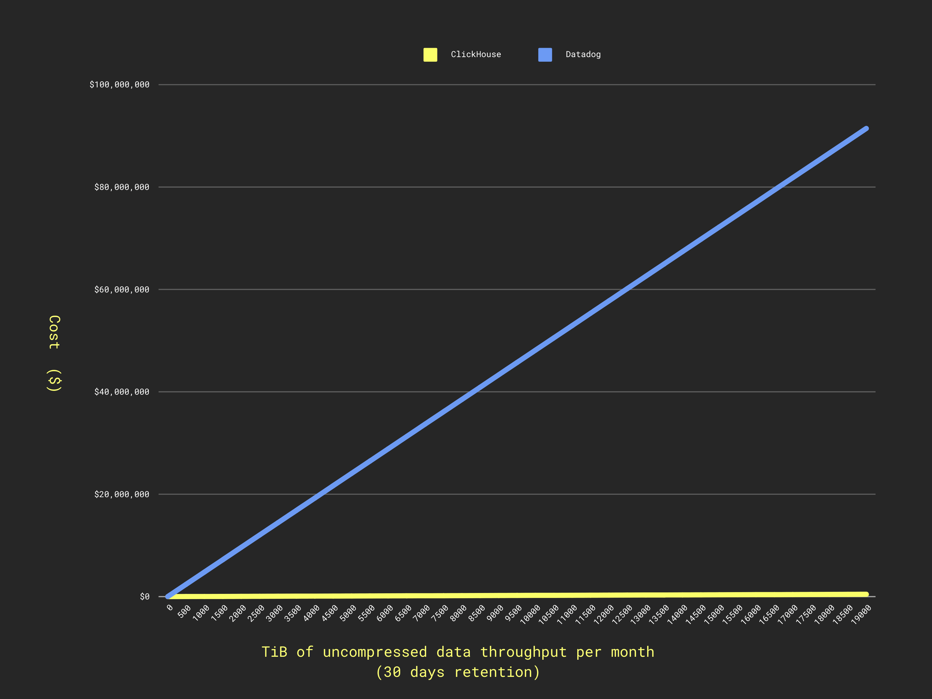
The yellow line here is actually ClickHouse! The 200x price ratio causes ClickHouse to appear as a horizontal line when overlaid on Datadog’s scale. Look closely, it's not quite flat :)
In reality, we store data for 6 months, with AWS LogHouse hosting 19 PiB of uncompressed logs. Importantly, however, this only impacts our storage cost and does not change the volume of infrastructure we use. This can be attributed to the use of S3 for separation of storage and compute. This means our query performance is slower if a linear scan is required, e.g. during historical analysis. We accept this in favor of a lower overall price per TiB, as shown below:
(1.13 PiB (compressed) * 1048576 * 0.021) = $24,883 + $125000 ≈ $150,000
So $150,000 per month for 19.11 PiB of uncompressed logs or $7.66 per TiB.
Cost comparison
Given that we never seriously considered other solutions, such as Datadog or Elastic, as being even remotely competitive in price, it is difficult to say that we have saved a specific amount.
If we consider Datadog and limit retention to 30 days, we can estimate a price. Assuming we do not query (maybe a bit optimistic), we would incur $0.1 per GiB ingested. At our current event size (see earlier top metrics), 1 TiB equates to around 1.885B events. Datadog charges a further $2.50 per million log events per month.
Our cost per TiB uncompressed per month is therefore:
Cost ($) = Ingest + Retention = (T*1000*0.1) + (T*1885*2.5) = 100T+4712T=4812T
Or around $4,230 per TiB throughput uncompressed. This is over 200x more expensive than ClickHouse.
Performance
Our largest ClickHouse LogHouse cluster consists of 5 nodes, each with 200 GiB RAM and 57 cores and holds over 10 trillion rows, compressing the data over 17x times. With a cluster in each cloud region, we are currently hosting over 37 trillion rows and 19 PiB of data in LogHouse spread across 13 clusters/regions and 48 nodes.
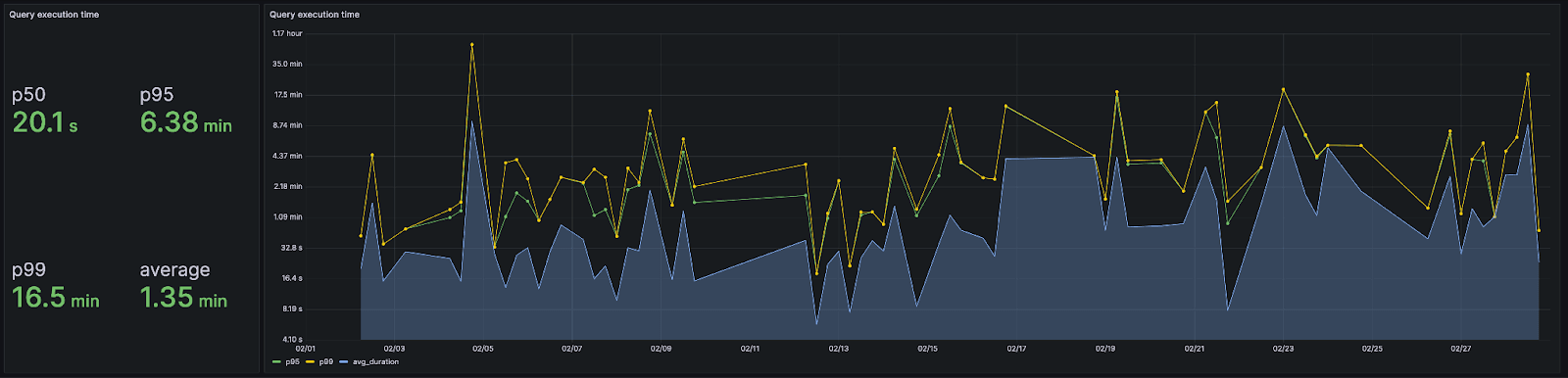
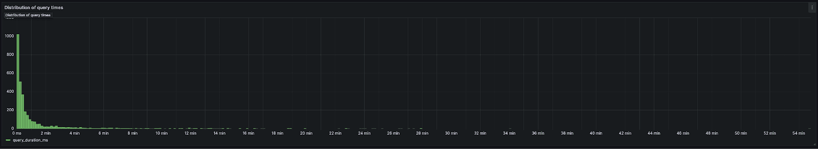
Our query latency is just over a minute. We note this performance is constantly improving and is heavily skewed by analysis queries (as suggested by the 50th percentile) performed by our core team which scan all 37 trillion rows aiming to identify a specific log pattern (e.g. to see if an issue a customer is encountering has ever been experienced by other users in the last 6 months). This is best illustrated through a histogram of query times.
Looking forward
From a ClickHouse core database development perspective, our Observability team is excited about a number of efforts. The most important of these being semi-structured data:
The recent efforts to move the JSON type to production-ready status will be highly applicable to our logging use case. This feature is currently being rearchitected, with the development of the Variant type providing the foundation for a more robust implementation. When ready, we expect this to replace our map with more strongly typed (i.e. not uniformly typed) metadata structures that are also possibly hierarchical.
From an integrations standpoint, we continue supporting the observability track by making sure to level up our integrations game across the pipeline. This translates into upgrading the ClickHouse OpenTelemetry exporter for collection and aggregation and an enhanced and opinionated Grafana plugin for ClickHouse.
Conclusion
In this post, we’ve shared the details of our journey to build a ClickHouse-powered logging solution that today stores over 19 PiB of data (1.13 PiB compressed) in our AWS regions alone.
We reviewed our architecture and key technical decisions behind this platform, in the hopes that this is useful to others who are also interested in building an observability platform with best-of-breed tools, rather than using an out-of-the-box service like Datadog.
And finally, we demonstrate that ClickHouse is at least 200x less expensive than Datadog for an observability workload like ours - the projected cost of Datadog for a 30-day retention period having been a staggering ~$26M per month!