Introduction
Earlier this year, we explored vector search capabilities in ClickHouse. While this predominantly focused on brute force linear techniques, where the search vector is compared to every vector in ClickHouse, which satisfies other filters, we also touched on the recently added emerging approximate nearest neighbor techniques. These are currently experimental in ClickHouse with support for Annoy and HNSW.
While a more traditional blog post might explore these algorithms, their implementation, and their use in ClickHouse, our CTO and founder Alexey Milovidov, believes most data problems can be solved with SQL. A few months ago, he presented an alternative approach to building a vector index using random projections and SQL during a meetup in Spain. In this post, we explore Alexey’s approach and test and evaluate its effectiveness.
A quick recap
Vector embeddings are a numerical representation of a concept composed of a series of floating point numbers (potentially thousands) representing a position in a high-dimensional space. These embeddings are usually produced by machine learning models such as Amazon’s Titan and can be created for any medium, such as text and images. Vectors that are close together in this high-dimensional space represent similar concepts. For three dimensions (the highest number of dimensions most people can comprehend), this can be visualized:
We explored this concept in detail in a previous post, including why this is useful. In vector search, the problem boils down to finding those vector embeddings in a large set that are similar to a search, or input, vector. This search vector will usually have been produced with a query using the same model. We are thus effectively finding vectors and, in turn, content, which is similar to our search query. This query again could be any medium.
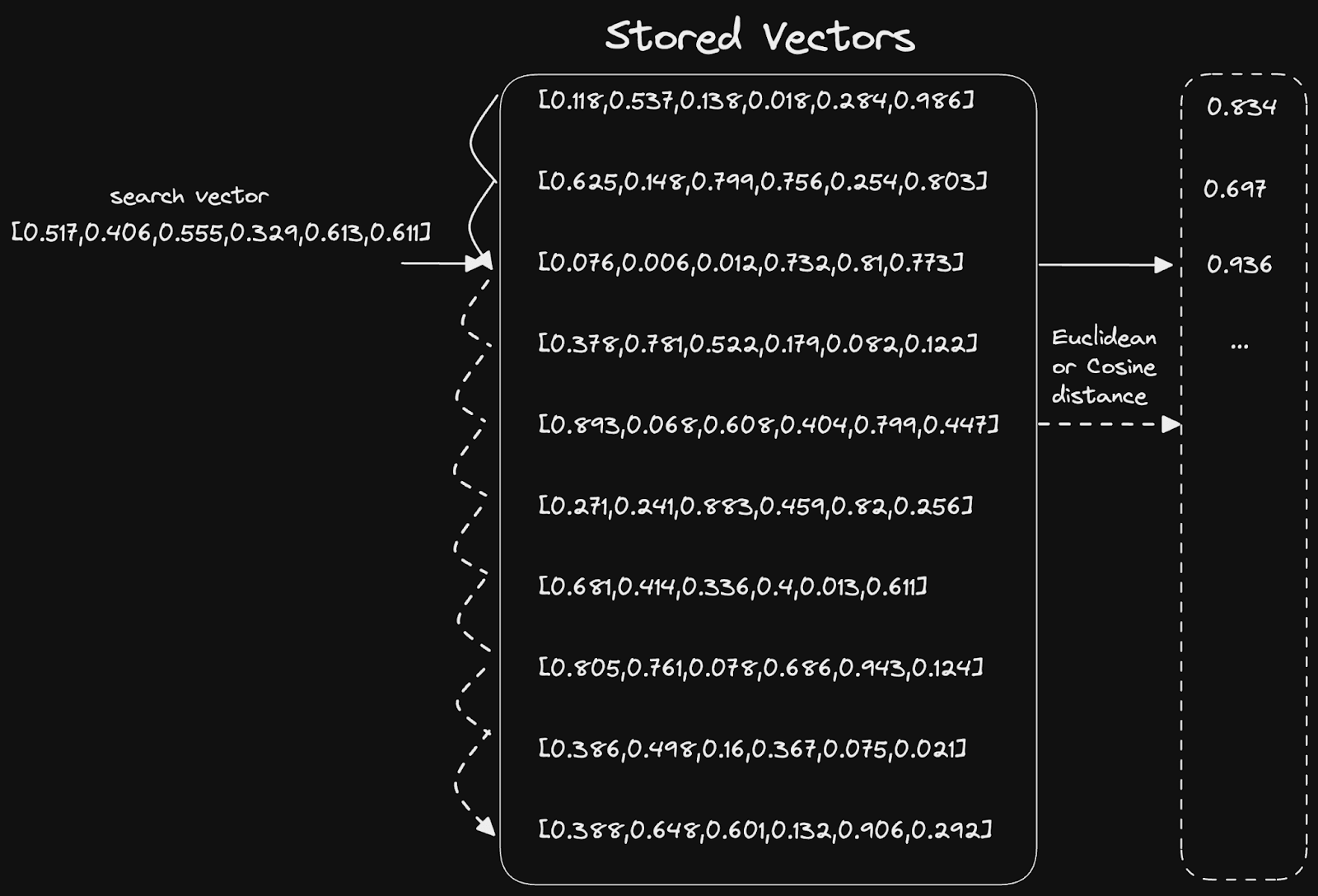
Similarly, in this context, this equates to distance or angle between two vectors. Math (usually cosine similarity or Euclidean distance) is used to compute these statistics and scales to N dimensions. The simplest solution to this problem is a simple linear scan:
Vector indices
While a linear scan can be very fast and sufficient, especially if highly parallelized, like in ClickHouse, there are data structures that can potentially reduce the O(n) complexity. These data structures, or vector indices, are exploited by approximation algorithms, which typically have to compromise between high recall (ratio of the number of relevant records retrieved to the total number of relevant records - assume we have a minimum similarity) and low latency.
These approximate algorithms are generally referred to as Approximate Nearest Neighbor (ANN). This naming alludes to the general problem of trying to find the nearest vector approximately.
Our linear scan approach has 100% recall but achieving acceptable latency at billions of rows can be challenging. In theory, these algorithms deliver lower latency responses at lower computational costs by sacrificing some recall. In effect, they return an approximate set of results, which may be sufficient provided a sufficient percentage of the “best results” are still present.
Typically, the quality of these algorithms is presented as a recall-latency curve or, alternatively, recall-QPS (queries per second) curve:
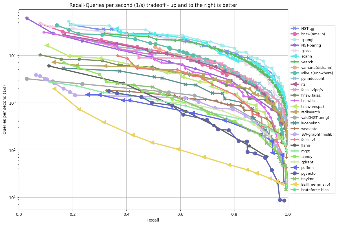 See ANN benchmarks
While this gives us a measure of performance, it usually represents an ideal setting. It fails to measure other important factors that emerge in production settings. For example, these algorithms also have varying degrees of support to allow vectors to be updated and whether they can easily be persisted to disk or must entirely operate in memory. Our simple linear scan suffers from none of these limitations.
While we recognize the value of algorithms such as HNSW (and hence we have added to ClickHouse), maybe we can revert to the basic principles of the problem and accelerate the searching of vectors while retaining the ability to easily update the set of vectors and not be bound by memory.
In this spirit, and because Alexey loves doing everything in SQL, he proposed a simple vector index based on Local Sensitive Hashing (LSH) and random projections.
Local sensitive hashing (LSH) with random projections
The core objective behind the following approach is to encode our vectors in a representation that reduces their dimensionality but preserves their distribution and locality to each other. With this lower dimensionality representation, we should be able to compute their similarity more efficiently (with respect to both memory and CPU). While we expect this to decrease the accuracy and recall of our similarity calculation (it becomes an estimate due to the information loss we take on by reducing dimensionality), we expect the quality to be sufficiently good while still benefiting from faster search times. As we’ll show, we can also combine this approach with an accurate distance calculation.
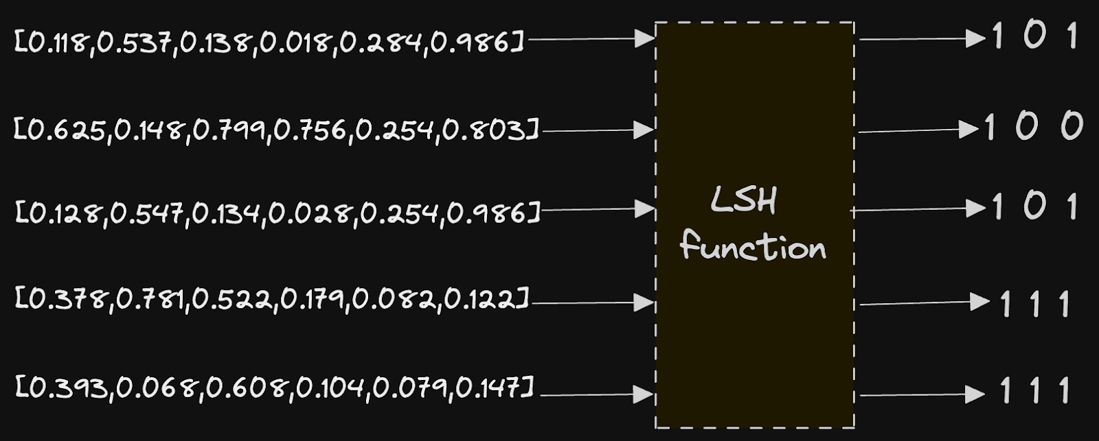
This approach relies on Local sensitive hashing or LSH. LSH is a hashing function that transforms data vectors to a lower dimension representation hash such that those that were close in their original domain are close in their resultant hash. This is effectively the opposite of a traditional hashing function, which would aim to minimize collisions and ensure this similarity was not preserved. In our case, our LSH is based on random projections with the resulting hash a bit sequence. Vectors that were close to the original space should have bit sequences with similar sequences of 1s and 0s.
The implementation here is relatively simple and brings us back to some high school mathematics. Assume our vectors are distributed roughly evenly in high dimensional space (see Benefits & Limitations if they aren't).
The goal is to partition our high dimensional space using N random hyperplanes, where N is configurable by the user. Once these planes are defined, we record which side of each plane a vector lies on, using a simple 1 or 0. This gives a bit set representation for each vector, with each bit position describing which side of a random plane the vector lies. Our bit sequence will thus be as long as the number of hyperplanes we select.
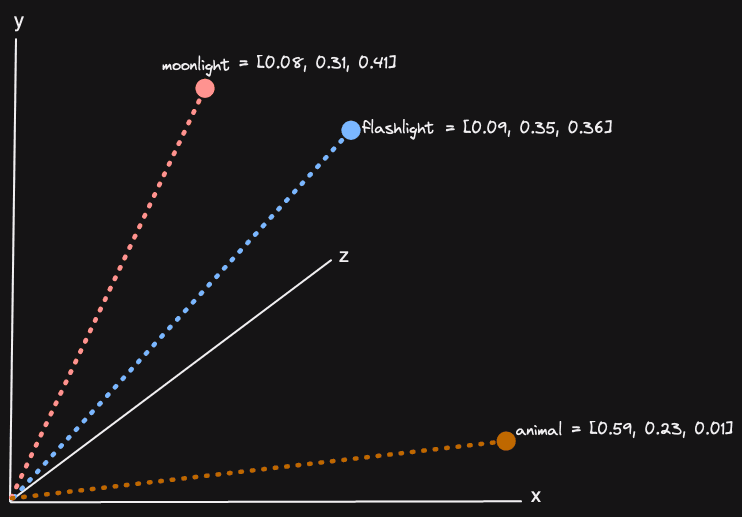
Let's look at a simplified example, assuming our vectors have only two dimensions. In this case, our hyperplanes are lines defined by a vector that passes through the origin 0,0.
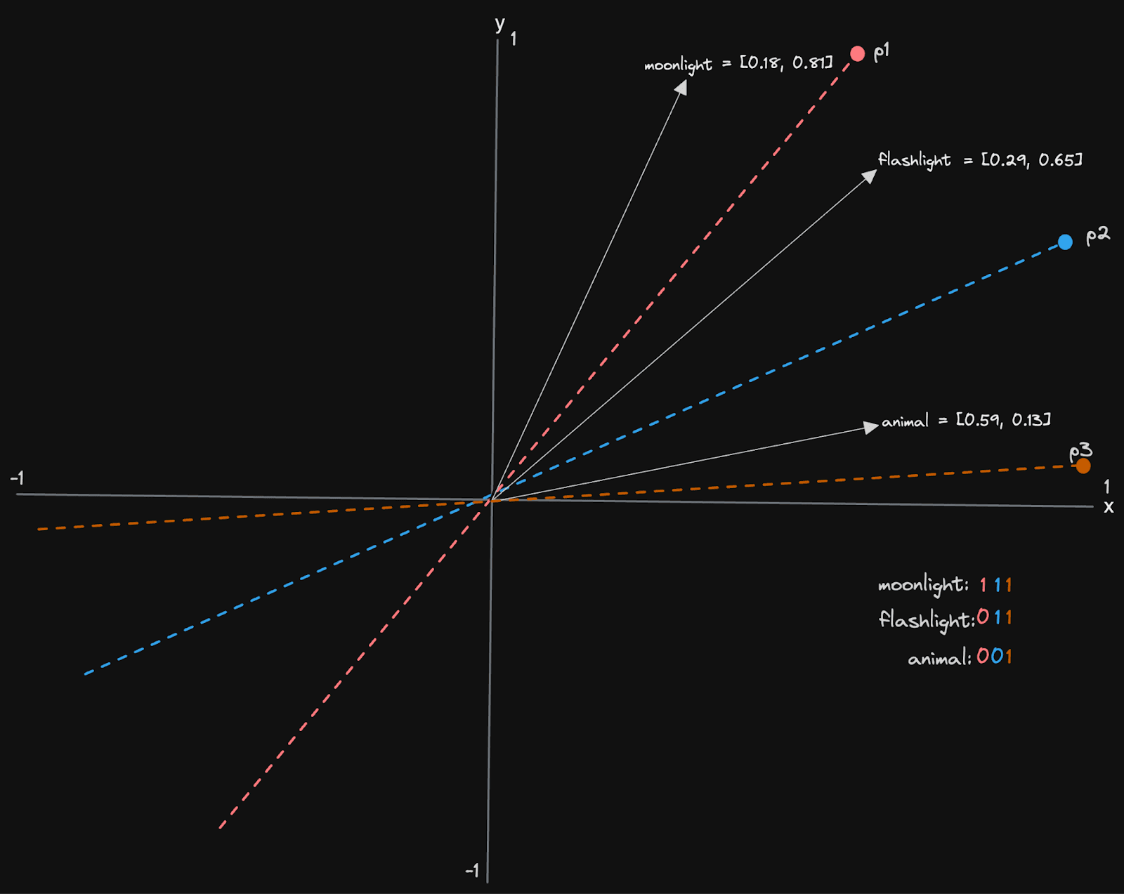
We have three planes, p1, p2, and p3, resulting in a 3-bit sequence for each vector. For each plane, we record if the vector is above or below the line, recording 1 for the former and 0 for the latter. The vector for “moonlight” sits above all lines and thus has a bit sequence of 111. “Flashlight” conversely is below p1 but above p2 and p3, resulting in 011. The above assumes that our vectors are within the unit space i.e. -1 to 1 (not always the case), and we have a notion of above and below a line (our example above might be intuitive but isn’t robust to all vectors in the space).
So, there are two resulting questions here: how do we compute whether a vector is above or below a line? And how do we select our lines?
To select our lines, we have a few options. If our vectors are normalized (-1 to 1), we can select a random point in the space sampled from a normalized distribution. We want these vectors to ideally be uniformly distributed over the surface of the space (effectively a unit sphere). To achieve this requires the use of the Norm. This point can be thought of as a random projection, which will pass through the origin, that defines our line and hyperplane in high-dimensional space by being its orthogonal/normal vector. This normal vector will be used for comparison against our line/plane to other vectors.
However, Alexey’s example assumes these vectors are not normalized. He thus uses a solution that aims to shift the vectors closer to the normalized space. While this will not create perfect uniformity to the normalized space, it does improve randomness. This is achieved by taking two random vectors in the space v1 and v2 and calculating the difference, labeling this as the normal ((v1 - v2)) vector, which defines the hyperplane. An offset or midpoint ((v1 + v2) / 2) of these vectors is also computed and used to effectively project vectors into this range for comparison to the normal by subtracting its value.
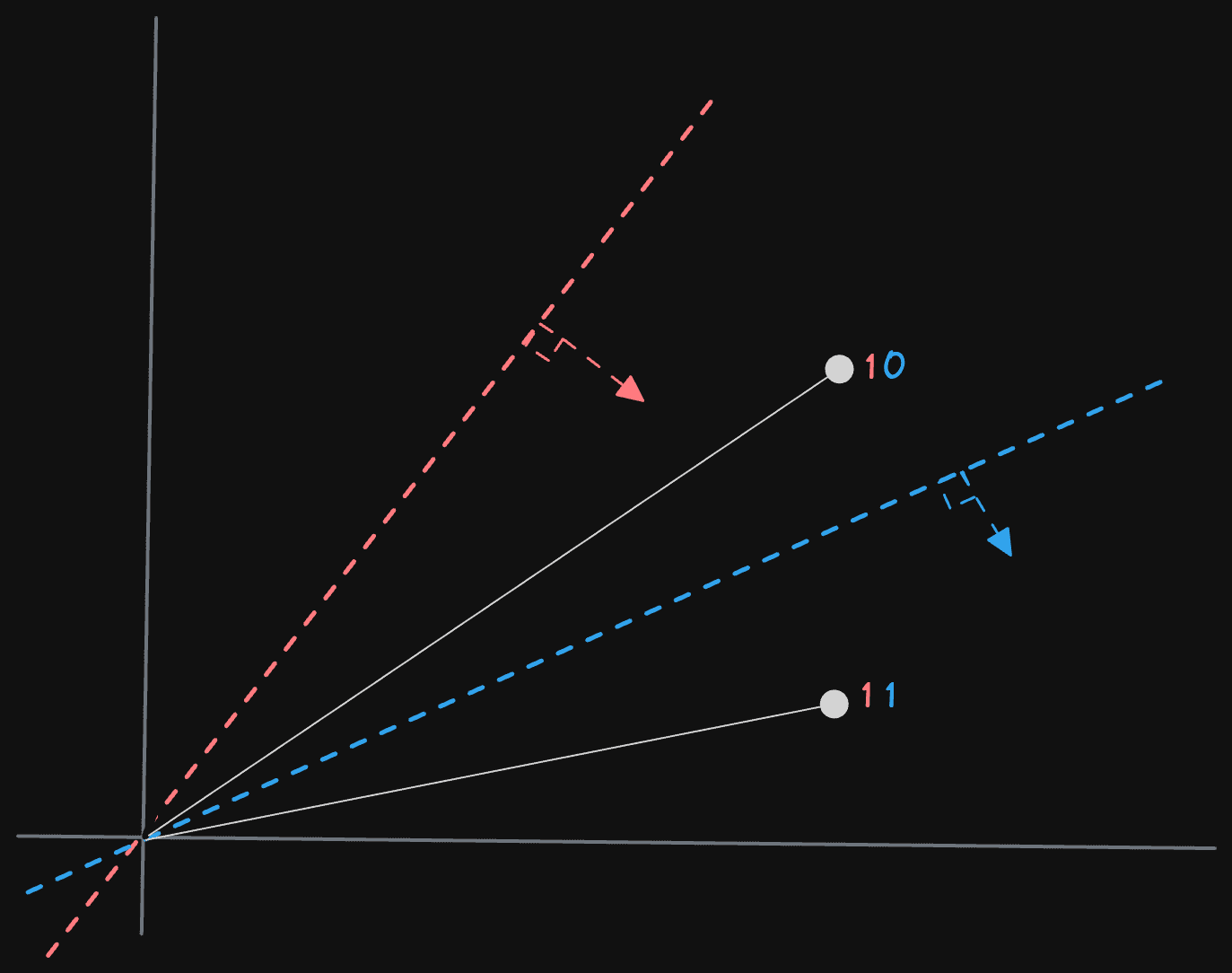
We can use a simple dot product with the normal vector defined above to calculate whether a vector v is above or below a line/plane. Calculated as the sum of the pairwise products of the corresponding components of the two vectors, this scalar value represents the similarity or alignment of the input vectors. If the vectors are pointed in the same direction, the value will be positive (with 1 indicating the same direction). Negative values mean they are in opposite directions (-1 exact opposite), whereas a value of 0 indicates they are orthogonal. We can thus use a positive value to indicate “above” the line and 0 or less as below.
For the non-normalized case above, we compute the dot product of normal and (v - offset). Moving forward, we’ll use this later approach since it is more robust but return to the simple case later to show the potential simpler syntax and slightly better performance.
Obviously, at this point, we have to imagine higher dimensions. The principle, however, remains the same. We choose two random points in the space, compute the vector between them, and record the midpoint. We use this plane information to compute whether points are orthogonal to the line.
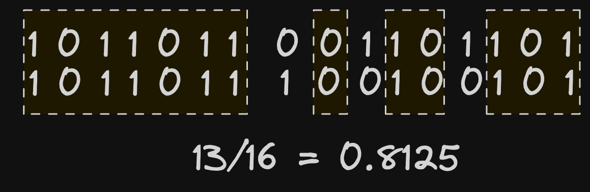
The above calculation has effectively acted as our LSH function and projected each vector into a lower dimensional space, resulting in a hash for each vector represented as a bit sequence. This sequence can be computed for every vector embedding in a table as well as for the embedding generated for a search query. We can, in turn, estimate the proximity of two vectors by comparing bit sequences. In theory, the more overlapping the bit sequences, the greater the number of shared sides of a hyperplane. A simple hamming distance, which measures the number of bits that are different, is sufficient here.
A pure SQL solution to ANN
Defining the planes
The above would be relatively simple to implement in Python or any programming language. However, ClickHouse is ideal for this task. Not only can we define the above using only a few lines of SQL, but we will take advantage of all the benefits of ClickHouse, including the ability to filter by metadata, aggregate, and not be bound to my memory. Inserting new vectors will also require us to compute a sequence for the row’s embeddings at insert time.
For our test dataset, we’ll use a test set from Glove consisting of 2.1m vectors trained from 840B CommonCrawl tokens. Each vector in this set has 300 dimensions and represents a word.
For our testing, we’ll use a ClickHouse Cloud instance with 16 cores.
We utilize the following schema for our target table. As discussed in previous posts, vectors in ClickHouse are just arrays of 32-bit floats.
CREATE TABLE glove
(
  `word` String,
  `vector` Array(Float32)
)
ENGINE = MergeTree
ORDER BY word
To load this dataset, we can use clickhouse local to extract the word and vector with string and array functions before piping the result to our client.
clickhouse local --query "SELECT trim(splitByChar(' ', line)[1]) as word, arraySlice(splitByChar(' ', line),2) as vector FROM file('glove.840B.300d.zip :: glove.840B.300d.txt','LineAsString') FORMAT Native" | clickhouse client --host <host> --secure --password '<password>' --query "INSERT INTO glove FORMAT Native"
Once loaded, we need to define our planes. We’ll store these in a table for fast lookup:
CREATE TABLE planes (
  normal Array(Float32),
  offset Array(Float32)
)
ENGINE = MergeTree
ORDER BY ()
The offset and normal here will be the midpoint and difference of two random vectors, as described earlier. We’ll populate this with a simple INSERT INTO SELECT. Note that at this point, we need to define the number of planes we wish to use to partition the space.
For the example below, we choose to use 128 planes to get started. This will result in a bit mash for each vector of 128 bits, which can be represented using a UInt128. To create 128 planes, we need 256 random vectors (2 for each plane). We group this random set using the expression intDiv(rowNumberInAllBlocks(), 2) and use the min and max functions to ensure a different vector is selected for each random point.
SELECT min(vector) AS v1, max(vector) AS v2
FROM
(
	SELECT vector
	FROM glove
	ORDER BY rand() ASC
	LIMIT 256
)
GROUP BY intDiv(rowNumberInAllBlocks(), 2)
The above gives us 128 rows, each with two random vectors, v1 and v2. We need to perform a vector difference to compute our' normal' column. A simple subtraction achieves this. The midpoint, called offset in the above table, can be computed using (v1 + v2)/2.
INSERT INTO planes SELECT v1 - v2 AS normal, (v1 + v2) / 2 AS offset
FROM
(
	SELECT
    	  min(vector) AS v1,
    	  max(vector) AS v2
	FROM
	(
    	  SELECT vector
    	  FROM glove
    	  ORDER BY rand() ASC
    	  LIMIT 256
	)
	GROUP BY intDiv(rowNumberInAllBlocks(), 2)
)

0 rows in set. Elapsed: 0.933 sec. Processed 2.20 million rows, 2.65 GB (2.35 million rows/s., 2.84 GB/s.)
Peak memory usage: 4.11 MiB.
In Alexey’s original talk, he used the expressions `arrayMap((x, y) -> (x - y), v1, v2)` and `arrayMap((x, y) -> ((x + y) / 2), v1, v2)` to compute the vector differences and midpoints. Vector arithmetic has subsequently been added to ClickHouse, allowing these operations to be constructed with simple `+`, `-` and `/`. This has the side benefit of being significantly faster!
Building bit hashes
With our planes created, we can proceed and create a bit of hash for each of our existing vectors. For this, we’ll create a new table, glove_lsh, using the earlier schema with a bits field of type UInt128 (as we have 128 planes). This will effectively be our index. Note that we order the table by column to accelerate later filtering operations. See Benefits & Limitations for more details on how this benefits filtering.
CREATE TABLE glove_lsh
(
  `word` String,
  `vector` Array(Float32),
  `bits` UInt128
)
ENGINE = MergeTree
ORDER BY (bits, word)
SETTINGS index_granularity = 128
We also lower our index_granularity for the table to 128. This was identified as an important optimization, as typically, we will return a small number of results and related vectors should be distributed in the same set of granules i.e. have similar bit hashes. Modifying this setting reduces our granule size and thus performs a secondary scan on fewer rows. As shown later, we may also wish to re-score vectors using a distance function (for a more accurate relevance score). This function is more computationally intensive, and reducing the number of rows on which it is executed will benefit response times.
To populate our table, we need to compute the bit mask for each vector. Note that we load 2m vectors in 100 seconds with our 16-core instance here.
INSERT INTO glove_lsh
WITH
   128 AS num_bits,
   (
       SELECT
           groupArray(normal) AS normals,
           groupArray(offset) AS offsets
       FROM
       (
           SELECT *
           FROM planes
           LIMIT num_bits
       )
   ) AS partition,
   partition.1 AS normals,
   partition.2 AS offsets
SELECT
   word,
   vector,
   arraySum((normal, offset, bit) -> bitShiftLeft(toUInt128(dotProduct(vector - offset, normal) > 0), bit), normals, offsets, range(num_bits)) AS bits
FROM glove
SETTINGS max_block_size = 1000

0 rows in set. Elapsed: 100.082 sec. Processed 2.20 million rows, 2.69 GB (21.94 thousand rows/s., 26.88 MB/s.)
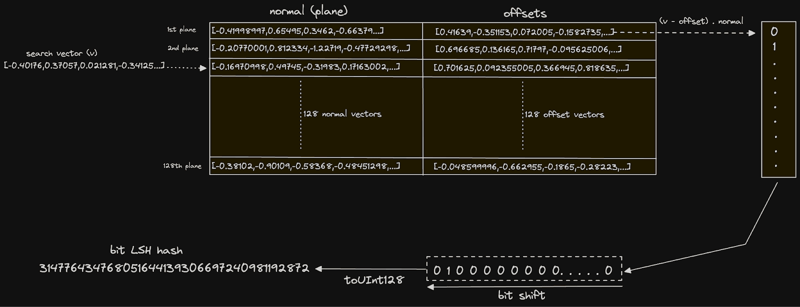
The first part of this query uses a CTE with the groupArray function to orientate our planes into a single row of two columns, each containing 128 vectors. These two columns hold all of our midpoints and difference vectors discussed earlier. In this structure, we are able to pass these into the expression responsible for computing the bit hash for each vector:
arraySum((normal, offset, bit) -> bitShiftLeft(toUInt128(dotProduct(vector - offset, normal) > 0), bit), normals, offsets, range(num_bits)) AS bits
This expression is executed for each row. The arraySum function sums the result of an array of 128 (num_bits) elements. This is performed through a lambda function which, for each array element i, computes (vector - offset) ⋅ normal where offset and normal are the vectors from the ith plane. This is the dot product calculation we described earlier and determines which side of the plane the vector lies. The result of this calculation is compared to 0, yielding a boolean, which we cast to UInt128 via the toUInt128 function. This value is bit-shifted by n places to the left, delivering a value where only the ith bit is set to 1 if the dot product yielded true and 0 otherwise. This ith bit effectively represents this vector relation to the ith plane. We sum these integers to give a decimal UInt128, the binary representation of which is our bit hash.
In the above insert, we reduce the
max_block_sizeto 1000. This is because the state of thearraySumfunction has a high memory overhead due to the planes being in memory. Large blocks with many rows can, therefore, be expensive. By reducing the block size, we reduce the number of rows and states processed at a time.
SELECT *
FROM glove_lsh
LIMIT 1
FORMAT Vertical

Row 1:
──────
word:   CountyFire
vector: [-0.3471,-0.75666,...,-0.91871]
bits:   6428829369849783588275113772152029372 <- how bit hash in binary
Once our index is created, we evaluate its size with the following query:
SELECT name, formatReadableSize(sum(data_compressed_bytes)) AS compressed_size,
	formatReadableSize(sum(data_uncompressed_bytes)) AS uncompressed_size,
	round(sum(data_uncompressed_bytes) / sum(data_compressed_bytes), 2) AS ratio
FROM system.columns
WHERE table LIKE 'glove_lsh'
GROUP BY name
ORDER BY name DESC

┌─name───┬─compressed_size─┬─uncompressed_size─┬─ratio─┐
│ word   │ 8.37 MiB    	   │ 12.21 MiB     	   │  1.46 │
│ vector │ 1.48 GiB    	   │ 1.60 GiB      	   │  1.08 │
│ bits   │ 13.67 MiB   	   │ 21.75 MiB     	   │  1.59 │
└────────┴─────────────────┴───────────────────┴───────┘
Our bits column is over 100x smaller than our vector. The question is now whether this compressed representation of the space is faster to query...
Querying
Before using our index, let's test a simple brute force search using cosine distance (as recommended for glove) to provide a benchmark of absolute quality and what we can consider the authoritative results. In the example below, we search for words similar to the word "dog":
WITH
   'dog' AS search_term,
   (
       SELECT vector
       FROM glove
       WHERE word = search_term
       LIMIT 1
   ) AS target_vector
SELECT
   word,
   cosineDistance(vector, target_vector) AS score
FROM glove
WHERE lower(word) != lower(search_term)
ORDER BY score ASC
LIMIT 5


┌─word────┬──────score─┐
│ dogs    │ 0.11640698 │
│ puppy   │ 0.14147866 │
│ pet     │ 0.19425482 │
│ cat     │ 0.19831467 │
│ puppies │ 0.24826884 │
└─────────┴────────────┘

10 rows in set. Elapsed: 0.515 sec. Processed 2.21 million rows, 2.70 GB (2.87 million rows/s., 3.51 GB/s.)
Peak memory usage: 386.24 MiB.
In the interest of simplicity, we use our glove index to look up the result. In a real search scenario, it is unlikely our word would be in the index and need to generate the vector embedding e.g. using an
embedUDF function.
For the same query, we need to construct the bit hash above for our term using our index.For our hamming distance calculation between our target vector’s bit and those in each row, we use the bitHammingDistance function.
The use of the bitHammingDistance function for UInt128 requires ClickHouse 23.11. Users on earlier versions should use bitCount(bitXor(bits, target)) for hammingDistance on UInt128s.
WITH 'dog' AS search_term,
   (
       SELECT vector
       FROM glove
       WHERE word = search_term
       LIMIT 1
   ) AS target_vector,
   128 AS num_bits,
   (
       SELECT
           groupArray(normal) AS normals,
           groupArray(offset) AS offsets
       FROM
       (
           SELECT *
           FROM planes
           LIMIT num_bits
       )
   ) AS partition,
   partition.1 AS normals,
   partition.2 AS offsets,
   (
       SELECT arraySum((normal, offset, bit) -> bitShiftLeft(toUInt128(dotProduct(target_vector - offset, normal) > 0), bit), normals, offsets, range(num_bits))
   ) AS target
SELECT word
FROM glove_lsh WHERE word != search_term
ORDER BY bitHammingDistance(bits, target) ASC
LIMIT 5

┌─word─────┐
│ animal   │
│ pup 	   │
│ pet 	   │
│ kennel   │
│ neutered │
└──────────

5 rows in set. Elapsed: 0.086 sec. Processed 2.21 million rows, 81.42 MB (25.75 million rows/s., 947.99 MB/s.)
Peak memory usage: 60.40 MiB.
A lot faster! The results are different from the exact results returned by the cosineDistance function but seem to make sense largely.
The quality returned by this distance estimation will likely vary on the vector space itself and how well the random places partition it. There are also cases where an estimation of quality is insufficient. Should quality be poor, or we need a more precise ordering, this index can also be used to pre-filter the result set before the matching results are rescored and possibly restricted to those that satisfy a threshold. This is a common technique and, historically, the approach in many traditional search systems where a term lookup is used, and a window is rescored with a vector (or other relevance) function.
WITH
   'dog' AS search_term,
   (
       SELECT vector
       FROM glove
       WHERE word = search_term
       LIMIT 1
   ) AS target_vector,
   128 AS num_bits,
   (
       SELECT
           groupArray(normal) AS normals,
           groupArray(offset) AS offsets
       FROM
       (
           SELECT *
           FROM planes
           LIMIT num_bits
       )
   ) AS partition,
   partition.1 AS normals,
   partition.2 AS offsets,
   (
       SELECT arraySum((normal, offset, bit) -> bitShiftLeft(toUInt128(dotProduct(target_vector - offset, normal) > 0), bit), normals, offsets, range(num_bits))
   ) AS target
SELECT
   word,
   bitHammingDistance(bits, target) AS approx_distance,
   cosineDistance(vector, target_vector) AS score
FROM glove_lsh
PREWHERE approx_distance <= 5
WHERE word != search_term
ORDER BY score ASC
LIMIT 5

┌─word───┬─approx_distance─┬──────score─┐
│ dogs   │           	4  │ 0.11640698 │
│ pet	 │           	3  │ 0.19425482 │
│ cat	 │           	4  │ 0.19831467 │
│ pup	 │           	2  │ 0.27188122 │
│ kennel │           	4  │  0.3259402 │
└────────┴─────────────────┴────────────┘

5 rows in set. Elapsed: 0.079 sec. Processed 2.21 million rows, 47.97 MB (28.12 million rows/s., 609.96 MB/s.)
Peak memory usage: 32.96 MiB.
So we’ve achieved a 10x speedup in performance and retained quality! An astute reader will have noticed the filter by the value of 5 - effectively, the number of bits that are different. This is within a maximum range of 128. How did we select this value?
Trial and error. This value should be robust across different search terms but will depend on the distribution of vectors in your space. A value that is too high and insufficient rows will be filtered prior to distance scoring, providing minimal performance benefit. Too low a value, and the desired results will be filtered out. A query to show the distribution of values can be helpful here. This distribution is normal (more specifically binomial):
WITH
   'dog' AS search_term,
   (
       SELECT vector
       FROM glove
       WHERE word = search_term
       LIMIT 1
   ) AS target_vector,
   128 AS num_bits,
   (
       SELECT
           groupArray(normal) AS normals,
           groupArray(offset) AS offsets
       FROM
       (
           SELECT *
           FROM planes
           LIMIT num_bits
       )
   ) AS partition,
   partition.1 AS normals,
   partition.2 AS offsets,
   (
       SELECT arraySum((normal, offset, bit) -> bitShiftLeft(toUInt128(dotProduct(target_vector - offset, normal) > 0), bit), normals, offsets, range(num_bits))
   ) AS target
SELECT
    bitCount(bitXor(bits, target)) AS approx_distance,
    bar(c,0,200000,100) as scale,
    count() c
FROM glove_lsh
GROUP BY approx_distance ORDER BY approx_distance ASC

┌─approx_distance─┬──────c─┬─scale─────────────────────────────────────────────────────────────────────────┐
│           	0 │  	 1 │                                                                           	   │
│           	2 │  	 2 │                                                                           	   │
│           	3 │  	 2 │                                                                           	   │
│           	4 │ 	10 │                                                                           	   │
│           	5 │ 	37 │                                                                           	   │
│           	6 │	   106 │                                                                           	   │
│           	7 │	   338 │ ▏                                                                         	   │
│           	8 │	   783 │ ▍                                                                         	   │
│           	9 │   1787 │ ▉                                                                         	   │
│          	   10 │   3293 │ █▋                                                                        	   │
│          	   11 │   5735 │ ██▊                                                                       	   │
│          	   12 │   8871 │ ████▍                                                                     	   │
│          	   13 │  12715 │ ██████▎                                                                   	   │
│          	   14 │  17165 │ ████████▌                                                                 	   │
│          	   15 │  22321 │ ███████████▏                                                              	   │
│          	   16 │  27204 │ █████████████▌                                                            	   │
│          	   17 │  32779 │ ████████████████▍                                                         	   │
│          	   18 │  38093 │ ███████████████████                                                       	   │
│          	   19 │  44784 │ ██████████████████████▍                                                   	   │
│          	   20 │  51791 │ █████████████████████████▉                                                	   │
│          	   21 │  60088 │ ██████████████████████████████                                            	   │
│          	   22 │  69455 │ ██████████████████████████████████▋                                       	   │
│          	   23 │  80346 │ ████████████████████████████████████████▏                                 	   │
│          	   24 │  92958 │ ██████████████████████████████████████████████▍                           	   │
│          	   25 │ 105935 │ ████████████████████████████████████████████████████▉                     	   │
│          	   26 │ 119212 │ ███████████████████████████████████████████████████████████▌              	   │
│          	   27 │ 132482 │ ██████████████████████████████████████████████████████████████████▏       	   │
│          	   28 │ 143351 │ ███████████████████████████████████████████████████████████████████████▋  	   │
│          	   29 │ 150107 │ ███████████████████████████████████████████████████████████████████████████   │
│          	   30 │ 153180 │ ████████████████████████████████████████████████████████████████████████████▌ │
│          	   31 │ 148909 │ ██████████████████████████████████████████████████████████████████████████▍   │
│          	   32 │ 140213 │ ██████████████████████████████████████████████████████████████████████    	   │
│          	   33 │ 125600 │ ██████████████████████████████████████████████████████████████▊           	   │
│          	   34 │ 106896 │ █████████████████████████████████████████████████████▍                    	   │
│          	   35 │  87052 │ ███████████████████████████████████████████▌                              	   │
│          	   36 │  66938 │ █████████████████████████████████▍                                        	   │
│          	   37 │  49383 │ ████████████████████████▋                                                 	   │
│          	   38 │  35527 │ █████████████████▊                                                        	   │
│          	   39 │  23526 │ ███████████▊                                                              	   │
│          	   40 │  15387 │ ███████▋                                                                  	   │
│          	   41 │   9405 │ ████▋                                                                     	   │
│          	   42 │   5448 │ ██▋                                                                       	   │
│          	   43 │   3147 │ █▌                                                                        	   │
│          	   44 │   1712 │ ▊                                                                         	   │
│          	   45 │	   925 │ ▍                                                                         	   │
│          	   46 │	   497 │ ▏                                                                         	   │
│          	   47 │	   245 │                                                                           	   │
│          	   48 │	   126 │                                                                           	   │
│          	   49 │    66  │                                                                           	   │
│          	   50 │    46  │                                                                           	   │
│          	   51 │    16  │                                                                           	   │
│          	   52 │    6   │                                                                           	   │
│          	   53 │    5   │                                                                           	   │
│          	   54 │    3   │                                                                           	   │
│          	   55 │    6   │                                                                           	   │
│          	   56 │    1   │                                                                           	   │
│          	   60 │    1   │                                                                               │
└─────────────---─┴─-──────┴───────────────────────────────────────────────────────────────────────────────┘

57 rows in set. Elapsed: 0.070 sec. Processed 2.21 million rows, 44.11 MB (31.63 million rows/s., 630.87 MB/s.)
The normal distribution is apparent here, with most words having a distance of around 30 bits. Here, we can see that even a distance of 5 actually limits our filtered results to 52 (1+2+2+10+37).
How robust is this distance limit across other queries? Below, we show the results for various search terms and approaches: (1) if we order by cosine distance with a brute force search, (2) ordering by hamming distance, (3) filtering by a distance of 5 and reordering by cosine distance (4) filtering by a distance of 10 and reordering by cosine distance. For each of these approaches, we provide the response time.
| search word | ORDER BY cosine | Response Time (s) | ORDER BY hamming distance | Response Time (s) | WHERE distance <= 5 ORDER BY cosine | Response Time (s) | WHERE distance <= 10 ORDER BY cosine | Response Time (s) |
|---|---|---|---|---|---|---|---|---|
| cat | cats kitten dog kitty pet | 0.474 | animal pup pet abusive kennel | 0.079 | dog kitty petfeline pup | 0.055 | cats kittendog kitty pet | 0.159 |
| frog | frogstoad turtle monkey lizard | 0.480 | peacock butterfly freshwater IdahoExterior terrestrial | 0.087 | butterflypeacockfreshwater | 0.073 | frogstoadturtlemonkey lizard | 0.101 |
| house | houses home apartment bedroom residence | 0.446 | People other laughing Registered gyrating | 0.080 | oneput areahadeveryone | 0.063 | houseshomeresidencehomes garage | 0.160 |
| mouse | micerat cursor keyboard rabbit | 0.499 | operational upheld Foley Mouse redundant | 0.073 | statusredundantwebcamsoperational digger | 0.045 | rat cursorhamsterrodenttyping | 0.141 |
| table | tables diningchairs chairdesk | 0.488 | oven xb saki truck ids chairs | 0.083 | oven | 0.068 | tableschairschairsofafurniture | 0.117 |
A few observations here:
- Ordering by hamming distance is around 6x faster than a simple brute force cosine distance search. However, result quality suffers significantly and is unlikely to be robust for reasons we’ll explain later.
- Filtering to a distance of 5 and reordering by cosine distance improves result quality over ordering by hamming distance. Performance is also superior, with response time up to 10 times faster than a brute-force search. However, the quality of results does not appear robust across all our search terms, prompting us to increase the minimum distance to 10.
- Filtering by a distance of 10 and reordering by cosine distance delivers consistently quality results. This approach delivers a 4x speed up over standard cosine distance.
Simpler planes
Our previous plane creation using a midpoint was relatively complex. As mentioned earlier, if our vectors are normalized (as is the case with glove), plane creation can be as simple as generating random points in the space that represent their normal vector. These need to be normalized between a value of -1 and 1 and selected from a normal distribution i.e. we effectively want to sample points uniformly from a unit sphere. Mathematically, this requires us to use norm of a vector, available in ClickHouse as the L2Norm function. The following INSERT INTO generates 128 points/planes on a unit sphere, each with 300 dimensions, using the randNormal and L2Norm functions in ClickHouse. There is some complexity here with the use of array functions - we leave this as an exercise for the user to decompose in the interests of post-brevity.
INSERT INTO planes_simple SELECT projection / L2Norm(projection) AS projection
FROM
(
    SELECT arrayJoin(arraySplit((x, y) -> y, groupArray(e), arrayMap(x -> ((x % 300) = 0), range(128 * 300)))) AS projection
    FROM
    (
        SELECT CAST(randNormal(0, 1), 'Float32') AS e
        FROM numbers(128 * 300)
    )
)
In this case, our planes consist of only a single point. This simplifies the query required to populate our table glove_lsh_simple with bit hashes. This simplification significantly improves insert time - now only 43 seconds (down from 100 seconds).
INSERT INTO glove_lsh_simple
WITH
    128 AS num_bits,
    (
        SELECT groupArray(projection) AS projections
        FROM
        (
            SELECT *
            FROM planes_simple
            LIMIT num_bits
        )
    ) AS projections
SELECT
    word,
    vector,
    arraySum((projection, bit) -> bitShiftLeft(toUInt128(dotProduct(vector, projection) > 0), bit), projections, range(num_bits)) AS bits
FROM glove
SETTINGS max_block_size = 1000

0 rows in set. Elapsed: 43.425 sec. Processed 2.20 million rows, 2.69 GB (50.57 thousand rows/s., 61.95 MB/s.)
Querying is also more straightforward and yields comparable results:
WITH
    'dog' AS search_term,
    (
        SELECT vector
        FROM glove
        WHERE word = search_term
        LIMIT 1
    ) AS target_vector,
    128 AS num_bits,
    (
        SELECT groupArray(projection) AS projections
        FROM
        (
            SELECT *
            FROM planes_simple
            LIMIT num_bits
        )
    ) AS projections,
    (
        SELECT arraySum((projection, bit) -> bitShiftLeft(toUInt128(dotProduct(target_vector, projection) > 0), bit), projections, range(num_bits))
    ) AS target
SELECT word
FROM glove_lsh_simple
WHERE word != search_term
ORDER BY bitCount(bitXor(bits, target)) ASC
LIMIT 5

┌─word────┐
│ dogs    │
│ puppy   │
│ pet     │
│ doggy   │
│ puppies │
└─────────┘

5 rows in set. Elapsed: 0.066 sec. Processed 2.21 million rows, 81.26 MB (33.63 million rows/s., 1.24 GB/s.)
Peak memory usage: 53.71 MiB.
Notice we also get a small performance boost here due to a reduction in query complexity.
Benefits & limitations
This approach has a number of advantages over more complex ANN algorithms such as HNSW. We have shown that when coupled with rescoring over a window, we retain relevance accuracy with a decent speedup - around 4x. The results above also show our queries have very low memory overhead - around 50MiB. While this can be attributed to ClickHouse not storing all bit sets in memory, the index representation is also very efficient, with only 128 bits per vector. This approach also doesn’t require the index to be held in memory, with a very compact representation on disk, as shown below:
SELECT
    table,
    name,
    formatReadableSize(sum(data_compressed_bytes)) AS compressed_size,
    formatReadableSize(sum(data_uncompressed_bytes)) AS uncompressed_size
FROM system.columns
WHERE table = 'glove_lsh'
GROUP BY table, name

┌─table─────┬─name───┬─compressed_size─┬─uncompressed_size─┐
│ glove_lsh │ word   │ 8.37 MiB        │ 12.21 MiB         │
│ glove_lsh │ vector │ 1.48 GiB        │ 1.60 GiB          │
│ glove_lsh │ bits   │ 13.67 MiB       │ 21.75 MiB         │
└───────────┴────────┴─────────────────┴───────────────────┘

5 rows in set. Elapsed: 0.024 sec.
We can see from the above that our bits column (effectively our index) consumes around 13MiB when compressed on disk, compared to the 1.5GiB required for storage of the vectors. Furthermore, adding additional rows is also trivial and computationally cheap - we compute our bits column at insert time. Finally, this approach lends itself to ClickHouse’s parallel execution model as well as being easy to distribute. This can be achieved by adding more cores to a node (i.e. scaling vertically) or by sharding the data across nodes. Alternatively, in ClickHouse Cloud, where only a single copy of the data is held in object storage, and compute is separated from storage, users can scale their nodes dynamically. Any of these approaches allow the work to be parallelized in order to either accelerate queries or support higher QPS rates.
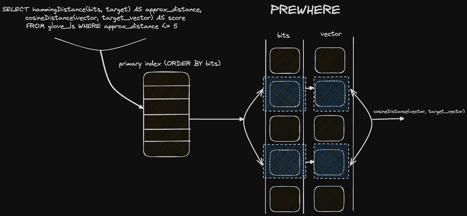
Finally, what may be interesting here is how this approach lends itself to ClickHouse specifically and its columnar structure on disk. Astute readers will have noticed we ordered our table by the bits column itself i.e. ORDER BY (bits, word). When filtering by a distance N and rescoring the top results, our query can exploit this ordering to speed up queries and avoid a complete linear scan. Our distance condition is provided in a PREWHERE condition, which effectively means the bit column is scanned first (in parallel) to identify the matching granules. Given the size of this column (around 13MiB), this can be done extremely quickly in ClickHouse's highly vectorized query pipeline. The vector column (significantly larger at 1.5GiB) will only be loaded and scanned for those granules that match our PREWHERE distance clause. This two-step filtering minimizes the data to be loaded and contributes to our performance.
While the above list of pros is compelling, there are some limitations. While we haven't rigorously evaluated recall, it is unlikely the above approach will be as effective as graph-based approaches such as HNSW. All ANN algorithms typically compromise as to how parametric they are and the size of the data structures used to divide and represent the high dimensional space. Algorithms that are graph-based are highly parametric and compute a granular representation of space.
Most importantly, these approaches invariably represent the notion of "neighbor" better. Our rather crude division of the space assumes no knowledge of the space and divides it into randomly generated planes (although our midpoint approach uses some information about the space, it's quite coarse). This would be perfectly fine if our vectors were evenly distributed in the space on each dimension. Unfortunately, in reality, they are not, with clusters of vectors being more common. If planes divide these clusters, then the proximity of two neighboring vectors can effectively be lost in the encoding. For example, consider the diagram below:
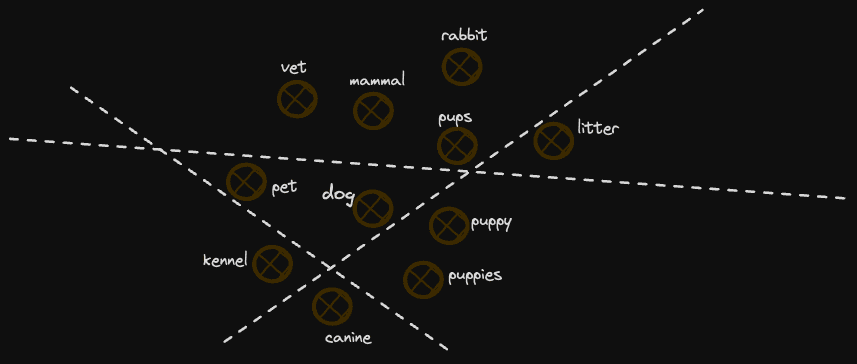
In this example, we lose some concepts similar to "dog" as they fall on opposite sides of dividing planes. As we increase the number of planes, this becomes less of an issue, e.g. it is unlikely a further 127 planes will all divide these 2 points. However, it is likely they will partition the space in an imperfect way, which leads to imperfect relevancy.
Furthermore, our measure of distance is rather crude and cannot be compared across searches. A specific distance measure has different notions of "closeness" or whether two vectors are "neighbors" depending on the location of the space. For example, a distance of 4 may represent a close neighbor in sparse areas of the space. Conversely, it may be meaningless in highly dense areas with many vectors.
A possible analogy here might be how the concept of a neighbor for people is relative to population density - a neighbor in New York is likely the person in the apartment opposite. In remote parts of Wyoming, it's probably 10s of miles. Graph-based algorithms such as HNSW address this problem by using a higher number of parameters and actually mapping out the space in more detail with a better division of the points, thus providing a superior measure of nearest neighbor. They are, however, more computationally expensive to update and persist on disk efficiently.
These factors make the distance metric we compute with our hamming distance coarse and an estimate only. Our rescoring approach using an exact cosine distance does help address this problem well while retaining the performance benefits.
Tuning
Finally, we will briefly address the question of how many hyperplanes we actually need and, thus, how large our bit hash should be. This would result in a longer blog post, but in summary, it depends on both the number of vectors and their dimensionality. Generally, more bits = better search quality (and recall) due to greater parametrization and partitioning of the space as well as fewer collisions in our LSH values at a cost of slower query performance.
For glove, we had 128 bits in our LSH, giving us effectively 2*128 = 3.4^1038 buckets in our hash. With 2 million vectors, this should result in a very low probability of collisions. The hash could possibly be reduced to 32 bits (represented via UInt32) with a sufficient number of buckets for minimal collisions. Our brief testing on the glove, however, suggested a value of 128 bits delivered the best result quality despite most buckets never being filled - the number of vectors per bucket can be determined with a simple aggregation and count on the bit column. While we have less than one vector per bucket on average with no collisions, increasing the resolution beyond the number required to avoid collisions improves the precision of the buckets and partitioning of our space.
Users with higher dimensional vectors may wish to experiment using more bits e.g. 256 bits via the UInt256. These larger spaces will require more planes to partition the vectors effectively. Be aware, however, that this will require more computational overhead as more bits will need to be compared. In summary, the number of bits/planes is often dataset-dependent and requires some testing (especially when combined with distance thresholds and rescoring), although 128 seems to be a good starting point.
Conclusion
In this post, we’ve looked at how ClickHouse users can create vector indices using only SQL to accelerate nearest-neighbor searches. More specifically, by creating random hyperplanes in high-dimensional space and computing bit sequences, we can estimate the distance between vectors using a hamming distance calculation. This approach potentially speeds up vector searches by 10x or 4x for exact matching. We have presented the pros and cons of this approach. Let us know whether you’ve found this useful and tried the approach on your own dataset!